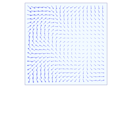
16.1 Vector Fields #

• A vector field in .$\mathbb{R}^3$ is a function .$\vec F$ on region .$E \in \mathbb{R}^3$ that assigns each point .$(x,y,z)$ a vector .$F(x,y,z)$
• .$\vec F$ is made up of component function: .$\vec F(x,y,z) = \langle P(x,y,z)\hat i, Q(x,y,z) \hat j, R(x,y,z) \hat k\rangle$
  • .$\vec F$ is continuos iff its component vectors are continuos
• .$\vec F$ is conservative (path taken doesn’t change work) iff potential function .$f(x,y,z)$ is a partial of .$\vec F$ $$\vec F = \nabla f$$
  • Notice that the gradient lines are always perpendicular to the level sets
    • If the function .$f$ is differentiable, .$\nabla f$ at a point is either zero or perpendicular to the level set of .$f$ at that point.
  • That is, that the gradient of a function is called a gradient field which is always conservative (the fundamental theorem of calculus for line integrals)
    • Conversely, a (continuous) conservative vector field is always the gradient of a function

16.2 Line Integrals #

• We know that the distance (length) normally is .$L = \int_a^b \sqrt{(dx/dt)^2 + (dy/dt)^2}\ dt$
• Over a vector field, we can think of the function being the density of the line (or height of particle). Therefore, we say .$ds = \int_a^b \sqrt{(dx/dt)^2 + (dy/dt)^2}\ dt$ and can write $$\int_C f(x,y) ds = \int_a^bf(x(t), y(t)) \cdot \sqrt{\bigg(\frac{dx}{dt}\bigg)^2 + \bigg(\frac{dy}{dt}\bigg)^2} dt$$ and for 3D in a slightly different form: $$\int_a^b f (\vec r (t) ) \vert \vec r’(t) \vert \Longrightarrow \int_a^b f(x(t), y(t), z(t)) \cdot \sqrt{x’(t)^2 + y’(t)^2 + z’(t)^2} dt$$
• We can write .$\vec a \to \vec b$ as .$(1-t)\vec a + t\vec b$ with .$t\in[0,1]$
• Just like usual, we can break up un-integrable smooth curves, i.e $$\int_a^z f (x,y) = \int_a^b f_1(x,y) + \int_b^c f_2(x,y) + \dots \int_{\dots}^z f_n(x,y)$$

wrt variable #

Opposed to the line integrals on .$f$ along .$C$ with respect to .$x$ both and .$y$, we can write line integral with respect to arc length as follows:

$$\int_C f(x,y) dx = \int_a^b f(x(t), y(t)) \cdot y’(t) dt$$ $$\int_C f(x,y) dy = \int_a^b f(x(t), y(t)) \cdot x’(t) dt$$

It frequently happens that line integrals with respect to .$x$ and .$y$ occur together which we abbr as

$$\int_C P(x,y)\ dx + \int_C Q(x,y)\ dy = \int_C P(x,y)\ dx + Q(x,y)\ dy$$

Orientation #

• When we parameterize a curve, we give it a direction
  • Positive: Enclosed region .$D$ is always on the left as we traverse curve .$C$ (counter-clockwise)
  • Negative: Enclosed region .$D$ is always on the right as we traverse curve .$C$ (clockwise)
• The orientation represents the direction of the line
  • The positive direction corresponding to increasing values of the parameter .$t$
  • Doesn’t matter for regular line integrals: .$\int_C f(x,y) ds = \int_C f(x,y) ds$
    • Deals with distance, .$ds$, which doesn’t depend on direction
  • Does matter for field line integrals: .$\int_C f(x,y) dx \neq \int_C f(x,y) dy$
    • Deals with displacement, .$dx/dy$, which depends on direction

Let .$\vec F$ be a continuous vector field defined on a smooth curve .$C$ given by a vector function .$\vec r(t), t\in[a,b]$. Then the line integral of .$\vec F$ along .$C$ is $$W = \int_C \vec F \cdot d\vec r = \int_a^b \vec F ( \vec r (t) ) \cdot (\vec r (t))’\ dt = \int_C \vec F \cdot \vec T\ ds$$

• .$\vec T(x,y,z)$ is the unit tangent vector at the point .$(x,y,z)$ on .$C$
• .$\vec F \cdot \vec T = \vec F(x,y,z) \cdot \vec T(x,y,z)$

• This equation says that work is the line integral with respect to arc length of the tangential component of the force.
• Then, for a non-conservative force i.e .$F = \langle P(x,y,z), Q(x,y,z), R(x,y,z) \rangle$ $$W = \int_a^b P(\vec r(t)) \cdot x’(t) + Q(\vec r(t)) \cdot y’(t) + R(\vec r(t)) \cdot z’(t)$$ $$ \Longrightarrow \int_C P\ dx + Q\ dy + R\ dz$$
• If we flip the curve…
  • …and integrate with respect to just .$x$ or .$y$ then the value flips: $$\int_{-C}f(x,y)\ dx = - \int_C f(x,y)\ dx$$
  • Since .$\Delta x$ and .$\Delta y$ change sign when we reverse the orientation of .$C$.

  • …and integrate with respect to arc length, the value of the line integral does not change when we reverse the orientation of the curve: $$\int_{-C}f(x,y)\ ds = \int_C f(x,y)\ ds$$
  • This is because .$\Delta s$ is always positive.

16.3 Fundamental Thm for Line Integrals #

Let .$C$ be a smooth curve given by the vector function .$\vec r (t), t\in[a,b]$. Let .$f$ be a differentiable function of two or three variables whose gradient vector .$\nabla f$ is continuous on .$C$. Then $$\int_C \nabla f \cdot d\vec r =\int_C \vec F \cdot d\vec r = f(\vec r(b) ) f(\vec r(a))$$

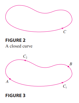
Independence of Path #

• Suppose .$C_1$ and .$C_2$ are two piecewise-smooth curves (which are called paths) that have the same initial point .$A$ and terminal point .$B$.
  • Therefore, .$\int_{C_1} \nabla f \cdot d\vec r = \int_{C_2} \nabla f \cdot d\vec r$ whenever .$\nabla f$ is continuous
  • In other words, line integrals of conservative vector fields are independent of path (they only depend on the start and end points)

Plane Curves #

.$\int_C \vec F \cdot d\vec r$ is independent of path in .$D$ iff .$\int_C \vec F \cdot d\vec r = 0$ for every closed path .$C$ in .$D$

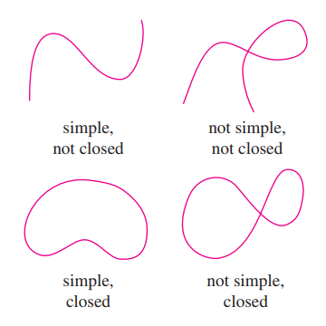
• Closed: A curve with the same end and start points: .$\vec r(b) = \vec r(a)$
• That is, only vector fields that are independent of path are conservative.

Space Curves #

• If .$\vec F (x,y) = P(x,y) \hat i + Q(x,y) \hat j$ is a conservative vector field, where .$P$ and .$Q$ have continuous first-order partial derivatives on a domain .$D$, then throughout .$D$ we have $$ \frac{\delta P}{\delta y} = \frac{\delta Q}{\delta x}$$
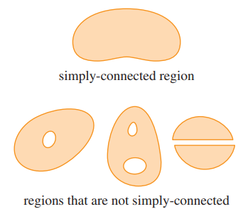
• The converse of the theorem above is true on only simple curves: curves that don’t intersect itself anywhere between its endpoints
• A simply-connected region in the plane is a connected region .$D$ such that every simple closed curve in .$D$ encloses only points that are in .$D$
  • Intuitively speaking, a simply-connected region contains no hole and can’t consist of two separate pieces.

.$\vec F = \langle P, Q \rangle$ is a conservative vector field on an open simply-connected region .$D$ iff both .$P$ and .$Q$ have continuous first-order partial derivatives and $$ \frac{\delta P}{\delta y} = \frac{\delta Q}{\delta x} \text{ throughout } D$$

16.4 Green’s Theorem #

Green’s Theorem: Let .$C$ be a positively oriented, piecewise-smooth, simple closed curve in the plane and let .$D$ be the region bounded by .$C$. If .$P$ and .$Q$ have continuous partial derivatives on an open region that contains .$D$, then $$\int_C \vec F \cdot d\vec r = \oint_C P\ dx + Q\ dy = \iint_D \bigg(\frac{\delta Q}{\delta x} - \frac{\delta P}{\delta y}\bigg) dA$$

• .$dA = dx\ dy = r \cdot dr\ d\theta = \dots$
• .$\vec F(x,y) = \langle P(x,y), Q(x,y)\rangle$
• .$\oint$ implies an integral over a closed curve

• The proof (for Green’s thm + remaining sections) is (are) too much for me to write out here, the book does a good job
  • One important takeaway is the the shape doesn’t have to be “nice” – we can break up any shape into parts that are either Type I or II. Even though we will have overlapping lines, they cancel one another out (leaving only the boundaries) because of orientation
• Green’s Theorem should be regarded as the counterpart of the Fundamental Theorem of Calculus for double integrals
  • Recall the Fundamental Theorem of Calculus is .$\int_a^b F’(x)\ dx = F(b) - F(a)$
  • In both cases there is an integral involving derivatives (.$F’, \delta Q/\delta x, \delta P/\delta y$) on the left side of the equation.
  • And in both cases the right side involves the values of the original functions (.$F, Q, P$) only on the boundary of the domain.
    • (In the one-dimensional case, the domain is an interval .$[a,b]$ whose boundary consists of just two points, .$a$ and .$b$.)

Application: Finding Area #

• Since the area of .$D$ is .$\iint_D 1 dA$, we wish to choose .$P$ and .$Q$ so that $$ \frac{\delta Q}{\delta x} - \frac{\delta P}{\delta y} = 1$$
• Some examples of .$P/Q$ combos are

  $$P(x,y)= 0$$ $$Q(x,y)= x$$ $$A = \oint_C x\ dy$$

  $$P(x,y)=-y$$ $$Q(x,y)= 0$$ $$A = -\oint_C y\ dx$$

  $$P(x,y)=-y/2$$ $$Q(x,y)= x/2$$ $$A = \frac{1}{2} \oint_C x\ dy - y\ dx$$

• Planimeters (a measuring instrument used to determine the area of an arbitrary two-dimensional shape) is an example of an application of Green Theorem
• We can also use Green’s to prove our last equation found in 16.3: $$\oint_C \vec F \cdot d \vec r = \oint_C P\ dx + Q\ dy = \iint_R \bigg( \frac{\delta Q}{\delta x} - \frac{\delta P}{\delta y}\bigg)\ dA = \iint_R 0\ dA = 0$$

  A curve that is not simple crosses itself at one or more points and can be broken up into a number of simple curves. We have shown that the line integrals of .$\vec F$ around these simple curves are all .$0$ and, adding these integrals, we see that .$\int_C \vec F \cdot d\vec r = 0$ for any closed curve .$C$. Therefore .$\int_C \vec F \cdot d\vec r$ is independent of path in .$D$. It follows that .$F$ is a conservative vector field.

16.5 Curl and Divergence #

• Recall that .$\nabla = \langle \frac{\delta}{\delta x} \frac{\delta}{\delta y} \frac{\delta}{\delta z} \rangle$
• 3b1b video going over this section

Curl #

• Vector of the rotation caused by the field at a given point $$\nabla \times \vec F(x,y,z) = \begin{bmatrix}\hat i & \hat j & \hat k\\ \frac{\delta}{\delta x} & \frac{\delta}{\delta y} & \frac{\delta}{\delta z}\\ P & Q & R\end{bmatrix} = \dots $$
• If .$\vec F$ is conservative then .$\text{curl($\vec F$) = 0}$
  • We know if .$\vec F$ is conservative then .$\vec F = \nabla f$ for some .$f(x,y,z)$
  • Crossing .$\nabla F$ with .$\nabla$ we get .$\langle \frac{\delta^2 f}{\delta y \delta z} - \frac{\delta^2 f}{\delta z \delta y}, \dots \rangle = \langle 0, 0,0 \rangle$

Divergence #

• If .$\vec F (x,y,z)$ is the velocity of a fluid (or gas), then .$\text{div}(\vec F (x,y,z))$ represents the net rate of change (wrt time) of the mass of fluid (or gas) flowing from the point .$(x,y,z)$ per unit volume.
  • In other words, .$\text{div}(\vec F (x,y,z))$ measures the tendency of the fluid to diverge from the point .$(x,y,z)$.
  • If .$\text{div}(\vec F (x,y,z)) = 0$, then .$F$ is said to be incompressible.
• Scalar of the amount of “flow” at a given point – how much does the field expand/contract at a given point? $$\nabla \cdot \vec F(x,y,z) = \langle \frac{\delta}{\delta x} \frac{\delta}{\delta y} \frac{\delta}{\delta z} \rangle \cdot \langle P, Q, R \rangle$$

• Fun fact: .$\text{(div(curl($\vec F$)))} = \nabla \cdot (\nabla \times \vec F)= 0$
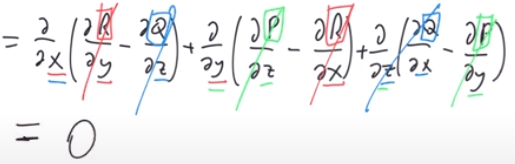
  • We can use this fact to find if there exists a vector field .$\vec G$ such that .$\text{curl($\vec G$)} = \vec H$ because .$\text{div(curl($\vec G$))} = \text{div($\vec H$)} = 0$

Vector Form of Green’s #

$$\oint_C \vec F \cdot d \vec r = \iint_D \text{(curl ($\vec F$))} \cdot \hat k\ dA = \bigg( \frac{\delta Q}{\delta x} - \frac{\delta P}{\delta y} \bigg) \hat k$$

• This equation expresses the line integral of the tangential component of .$\vec F$ along .$C$ as the double integral of the vertical component of .$\text{curl($\vec F$)}$ over the region .$D$ enclosed by .$C$.

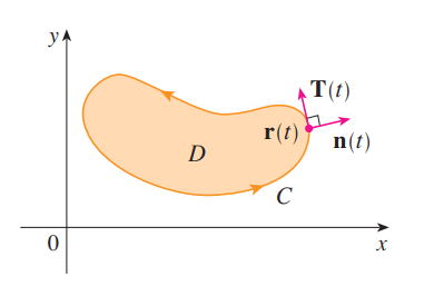
• We can write this using the normal component of .$\vec F$ too:
  • With .$\vec r(t) = \langle x(t), y(t) \rangle; t \in [a,b]$
  • Recall the unit tangent vector: .$\vec T(t) = \frac{1}{\vert \vec r ’ (t) \vert} \langle x’(t), y’(t) \rangle$
  • The outward unit normal vector to .$C$ is given by .$\vec n (t) = \frac{1}{\vert \vec r ’ (t) \vert} \langle y’(t), -x’(t) \rangle$
  • We can then evaluate $$\oint_C \vec F \cdot \vec n\ ds = \int_a^b (\vec F \cdot \vec n)(t) \vert \vec r’(t) \vert\ dt = \iint_D \bigg( \frac{\delta P}{\delta x} - \frac{\delta Q}{\delta y} \bigg)\ dA = \iint_D \text{div $\vec F (x,y)$}\ dA$$
  • This says that the line integral of the normal component of .$\vec F$ along .$C$ is equal to the double integral of the divergence of .$\vec F$ over the region .$D$ enclosed by .$C$.

16.6 Parametric Surfaces and Their Area #

Parametric Surfaces #

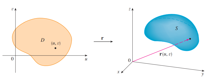
• Just like how we can describe curves with single parameter (variable) function .$\vec r(t)$, we can describe surfaces with a vector function .$\vec r(u,v) = \langle x(u,v), y(u,v), z(u,v) \rangle$
  • .$\vec r(u,v)$ is called a vector-valued function defined on a region .$D$ in the .$uv$-plane
  • .$x,y,z$ are the component functions of .$\vec r$, each of which have domain .$D$
• In general, a surface given as the graph of a function of .$x$ and .$y$, that is, with an equation of the form .$z = f(x,y)$, can always be regarded as a parametric surface by taking .$x$ and .$y$ as parameters and writing the parametric equations as .$x = x; y = y; z = f(x,y)$
  • E.x. the plane with point .$(x_0, y_0, z_0)$ and vectors .$\langle a,b,c \rangle$ .$\langle \alpha,\beta,\gamma \rangle$ is .$\vec r(u,v) = \langle x_0, y_0, z_0 \rangle + u\langle a,b,c \rangle + v\langle \alpha,\beta,\gamma \rangle$ or .$0 = (\langle x - x_0, y - y_0, z - z_0 \rangle) \cdot (\langle a,b,c \rangle \times \langle \alpha,\beta,\gamma \rangle)$

Surfaces of Revolution #

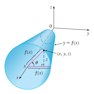
• We can write surfaces of revolution as parametric equations too
• Consider surface .$S$ obtained by rotating the curve .$y = f(x)$ about the .$x$-axis (with .$f(x) \geq 0$)
• Therefore, we get the following parameterization:

$$x = x$$

$$y = f(x)\cos\theta$$

$$z = f(x)\sin\theta$$

Tangent Planes #

• Employing the same method as before, we can find the tangent plane to a param surface .$S$ by finding the initial point and the normal vector
• Given some parameterization .$\vec r(u,v) = \langle x(u,v), y(u,v), x(u,v) \rangle$ and initial point .$P_0 = (x_0, y_0)$…
  1. Find point .$P_0$ by setting .$x(u,v) = x_0, y(u,v) = y_0, \dots$ and solving for .$u_0,v_0$
  2. Find normal vector .$\vec n$ by deriving to get, then cross, the parameterization: .$\vec n = \vec r_u \times \vec r_v$
     • If the normal vector isn’t zero, the tangent plane is at .$\vec n (u_0, v_0)$
     • If it is, then the surface .$S$ isn’t smooth (it is at a “corner”)
  3. The tangent plane can then be expressed as $$(\vec r_u \times \vec r_v)_{(u_0, v_0)} \cdot (\langle x,y,z \rangle - \langle x_0, y_0, z_0 \rangle)$$

Surface Area #

The image of the subrectangle .$R_{ij}$ is the patch .$S_{ij}$.

• Recall that the magnitude of the cross product is the area of a parallelogram formed by two vectors
• We can think of this as the jacobian of the transformation

If a smooth parametric surface .$S$ is given by the equation $$\vec r(u,v) = \langle x(u,v), y(u,v), z(u,v) \rangle; (u,v) \in D$$ and .$S$ is covered just once as .$(u,v)$ ranges throughout the parameter domain .$D$, then the surface area of .$S$ is $$A(S) = \iint_D \vert \vec r_u \times \vec r_v \vert\ dA$$ where $$\vec r_u = \langle \frac{\delta x}{\delta u}, \frac{\delta y}{\delta u}, \frac{\delta z}{\delta u} \rangle; \vec r_v = \langle \frac{\delta x}{\delta v}, \frac{\delta y}{\delta v}, \frac{\delta z}{\delta v} \rangle$$

Surface Area of the Graph of a Function #

• For the special case of a surface .$S$ with equation .$z = f(x,y)$, where .$(x,y)$ lies in .$D$ and .$f$ has continuous partial derivatives, we take .$x$ and .$y$ as parameters.
  • That is, the parametric equations are .$x = x; y = y; z = f(x,y)$
  • Therefore .$\vec r_x = \langle 1, 0, \frac{\delta f}{\delta x} \rangle; \vec r_y = \langle 0, 1, \frac{\delta f}{\delta y};$ and .$\vec n = \sqrt{1 + \frac{\delta f}{\delta x}^2 + \frac{\delta f}{\delta y}^2}$
  • Thus, the surface area becomes $$A(S) = \iint_D \sqrt{1 + \frac{\delta f}{\delta x}^2 + \frac{\delta f}{\delta y}^2}\ dA$$
• Notice the similarity between the surface area formula above and the arc length formula

16.7 Surface Integral #

Surface Integral #

• The relationship between surface integrals and surface area is much the same as the relationship between line integrals and arc length.
  • The arc length is a line integral where the density (or weight) function .$f(x,y,z) = 1$
    • That is, .$\int_C f(x,y,z)\ ds = \int_a^b f(\vec r(t)) \vert \vec r’(t) \vert$
  • Similarly, the surface area is found taking the surface integral with density function .$f(x,y,z) = 1$
    • That is, .$\iint_S 1\ dS = \iint_D \vert \vec r_u \times \vec r_v \vert\ dA = A(S)$
• If we define .$\vec r(u,v) = \langle x(u,v), y(u,v), z(u,v) \rangle; (u,v) \in D$ $$\iint_S f(x,y,z)\ dS = \iint_D f(\vec r(u,v)) \vert \vec r_u \times \vec r_v \vert\ dA$$

Graphs of Functions #

• Any surface .$S$ with equation .$z = g(x,y)$ can be regarded as a parametric surface with parametric equations

  $$x = x$$

  $$y = y$$

  $$z = g(x,y)$$

• Thus,

  $$\vec r_x = \bigg\langle 1, 0, \frac{\delta g}{\delta x}\bigg\rangle$$

  $$\vec r_y = \bigg\langle 0, 1, \frac{\delta g}{\delta y}\bigg\rangle$$

  $$\vec r_x \times \vec r_y = \bigg\langle -\frac{\delta g}{\delta x}, -\frac{\delta g}{\delta y}, 1\bigg\rangle$$

  $$\vec n = \sqrt{\bigg(\frac{\delta z}{\delta x}\bigg)^2 + \bigg(\frac{\delta z}{\delta y}\bigg)^2 + 1}$$

• Therefore, $$\iint_S f(x,y,z)\ dS = \iint_D f(x,y,g(x,y)) \sqrt{\bigg(\frac{\delta z}{\delta x}\bigg)^2 + \bigg(\frac{\delta z}{\delta y}\bigg)^2 + 1}\ dA$$
  • Similar formulas apply when it is more convenient to project .$S$ onto the .$yz$-plane or .$xz$-plane.

Oriented Surfaces #

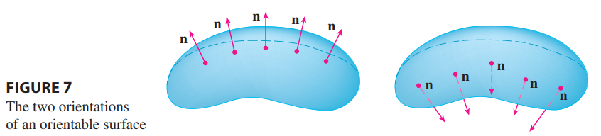
• With the exception of the Möbius strip, most surfaces are two-sided, meaning they’re Orientable surfaces
  • We start with a surface .$S$ that has a tangent plane at every point .$(x,y,z)$ on .$S$ (except at any boundary point).
  • There are two unit normal vectors .$\hat n_1$ and .$\hat n_2 = -\vec n_1$ at .$(x,y,z)$
  • If it is possible to choose a unit normal vector .$\hat n$ at every such point .$(x,y,z)$ so that .$\hat n$ varies continuously over .$S$, then .$S$ is called an oriented surface
    • The choice of .$\hat n$ provides .$S$ with an orientation.
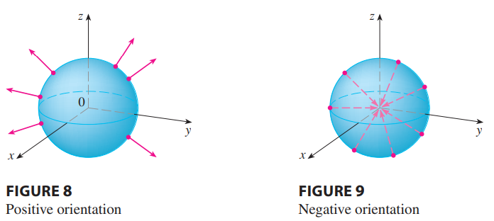
    • There are two possible orientations for any orientable surface
    • For a closed surface, the positive orientation has the normal vectors pointing outward and vis-versa

    

• If .$S$ is a smooth orientable surface given in parametric form by a vector function .$\vec r (u,v)$ then it is automatically supplied with the orientation of the unit normal vector $$\hat n = \frac{\vec r_u \times \vec r_v}{\vert \vec r_u \times \vec r_v \vert}$$
• E.x., going back to a surface .$z = g(x,y)$ given as the graph of .$g$, the normal unit vector is $$\hat n = \frac{\big\langle -\frac{\delta g}{\delta x}, -\frac{\delta g}{\delta y}, 1\big\rangle}{\sqrt{\big(\frac{\delta z}{\delta x}\big)^2 + \big(\frac{\delta z}{\delta y}\big)^2 + 1}}$$
  • Since the .$\hat k$-component is positive, this gives the upward orientation of the surface.

Surface Integrals of Vector Fields (Flux) #

If .$\vec F$ is a continuous vector field defined on an oriented surface .$S$ with unit normal vector .$\hat n$, then the surface integral of .$\vec F$ over .$S$ is $$\iint_S \vec F \cdot d\vec S = \iint_S \vec F \cdot \hat n \ dS = \iint_D \vec F \cdot (\vec r_u \times \vec r_v)\ dA$$ This integral is also called the flux of .$\vec F$ across .$S$.

• In words, the surface integral of a vector field .$\vec F$ over .$S$ is equal to the surface integral of its normal component over .$S$ (as previously defined).
• We can apply this to fluids:
  • Imagine a fluid with density .$\rho (x,y,z)$ and velocity field .$\vec v (x,y,z)$ flowing through .$S$.
  • Think of .$S$ as an imaginary surface that doesn’t impede the fluid flow, like a fishing net across a stream.
  • Then the rate of flow (mass per unit time) per unit area is .$\vec F = \vec v \rho$
  • The flux can be interpreted physically as the rate of flow through .$S$.

16.8 Stokes’ Theorem #

• Just as Green’s Theorem relates a double integral over a plane region .$D$ to a line integral around its plane boundary curve, Stokes’ Theorem relates a surface integral over surface .$S$ to a line integral around the boundary curve of .$S$ (which is a space curve)

  Stokes’ Theorem: Let .$S$ be an oriented piecewise-smooth surface that is bounded by a simple, closed, piecewise-smooth boundary curve .$C$ with positive orientation. Let .$\vec F$ be a vector field whose components have continuous partial derivatives on an open region in .$\mathbb{R}^3$ that contains .$S$. Then $$\int_C \vec F \cdot d \vec r = \iint_S \text{curl } \vec F \cdot d\vec S$$

• In words, Stokes’ Theorem says that the line integral around the boundary curve of .$S$ (some curve.$C$) of the tangential component of .$\vec F$ is equal to the surface integral over .$S$ of the normal component of the curl of .$F$
• This is since $$\int_C \vec F \cdot d \vec r = \int_C \vec F \cdot \vec T\ ds \ \ \ \text{ and }\ \ \iint_S \text{curl } \vec F \cdot d\vec S = \iint_S \text{curl } \vec F \cdot \hat n\ dS$$

16.9 Divergence Theorem #

Divergence Theorem: Let .$E$ be a simple solid region and .$S$ be the boundary surface of .$E$, given with positive (outward) orientation. Let .$\vec F$ be a vector field whose component functions have continuous partial derivatives on an open region that contains .$E$. Then $$\iint_S \vec F \cdot d\vec S = \iiint_E \text{div } \vec F\ dV$$

• In words, we can say that the Divergence Theorem says that (under the given conditions) the flux of .$\vec F$ across the boundary surface of .$E$ is equal to the triple integral of the divergence of .$\vec F$ over .$E$.