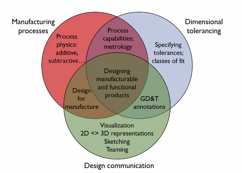
This class focuses on three main components – manufacturing processes, dimensional tolerances, and design communication – and how they interact with one another.
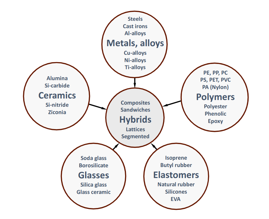
In this class we will consider multiple families of materials:
Materials choices influence performance
For example, consider the progress of the plane:
In 1903 the right brothers low-density wood with steel wire and silk
In 1935 the Douglas DC3 used aluminum alloy (since it became feasible to produce and manipulate)
Now the 2010
Boeing 787 Dreamliner is made up of 50 wt% composites 20 wt% aluminum 15 wt% titanium 20% lower fuel consumption per passenger mile
Composite materials are two(+) materials combined together to get best of both worlds, in aviation typically stiff/strong carbon fibers embed in tough/fatigue-resistant polymers.
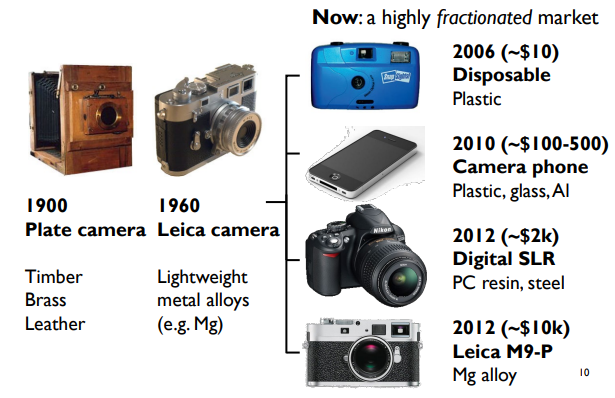
Materials choices influence market size
There isn’t always a best material; different materials fit different markets/needs
Opposite side of the coin: There may be multiple valid material choices for a particular function
Tolerancing is a formal way of specifying limits on the amount of dimensional variability allowable in manufactured parts
We need a range because measurements will never be 100% precise; we need to define an acceptable range
Some sources of variation
Human operator changes and/or errors
Tool wear
Environmental changes (temperature, humidity leads to tiny expansions / contractions)
Input material variability
Measurement error
Affordable mass-production relies on interchangeability of parts
When mating parts of given designs, it should not matter which specific parts
Therefore part dimensions must be consistent
But no manufacturing process is perfectly consistent
If you don’t understand the process of manufacturing and the capabilities of tools, then you will won’t know how to create manufacturable designs
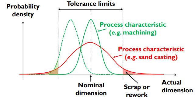
Tighter tolerances (closer tolerance limits) are generally more expensive to achieve
The solid green line shows an ideal process
The dotted green line shows the impact of an error shifting the distribution, shifting the tails to approach the tolerance upper / lower bound
The red line shows a unsuitable process (even if it’s calibrated accurately, the poor precision causes high variance that it’s not really feasible; however, if outside of the limits an additive (or less common subtractive) could be used to )
How E29 integrates manufacturing and tolerancing
#
Tighter tolerances are more expensive
The physics of a process determine how tight a tolerance is achievable and how much it costs
Therefore we need to understand how manufacturing processes work in order to:
Select a suitable process for the application
Specify reasonable tolerances
Geometric Dimensioning and Tolerancing: a graphical language for specifying tolerances robustly
We want to look at a process, look at tolerances, and figure out whether it’s worth to manufacture using this process
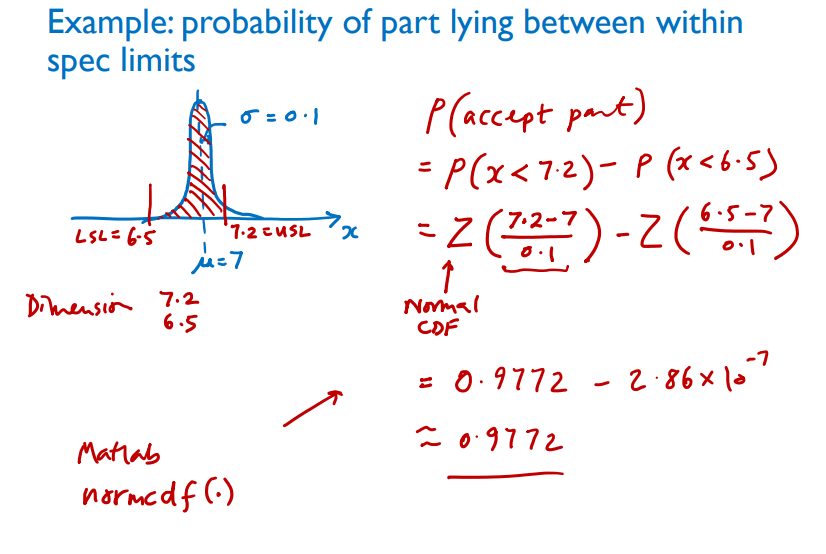
If you know the distribution of a process, you can work out the probability a given part satisfies spec limits.
There is no easy, exact analytical way to integrate the normal probability density function.
The probability that a randomly chosen member of a normally distributed population has a value .$\leq x$ is
$$\int_{-\infty}^x p(x)\ dx = P(x) = Z\bigg(\frac{x-\mu}{\sigma}\bigg) = \frac{1}{2}\bigg[1 + \text{erf}\bigg(\frac{x-\mu}{\sigma\sqrt{2}}\bigg)\bigg]$$
Six Sigma (6σ) is a set of techniques and tools for process improvement. […] A six sigma process is one in which 99.99966% of all opportunities to produce some feature of a part are statistically expected to be free of defects.
Specification limits are .$12\sigma$ apart. Here, 2 parts per billion lie outside specification limits if process is ‘in control’ (i.e. if mean output of process is centered between specification limits)
Arose because the cost of manufacturing, specifically the process that creates an error, has a cost. This cost can grow very large, very quickly, when mass-manufacturing.
You’re best off spending money improving the process so the distribution gets tighter
The alternative is either (1) accepting errors (resulting in faulty products) or (2) testing all components to ensure they are ‘good’ and tossing out the bad ones
Process capability: .$C_p = \frac{\text{USL - LSL}}{6\sigma}$
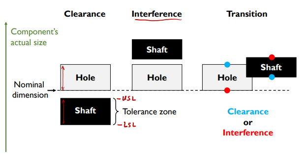
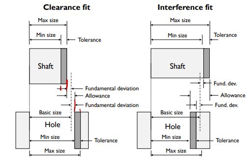
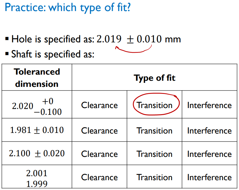
Clearance fit: designed with space left between two components
e.g. a shaft with a bearing need to have some give / free space
Interference (push) fit: designed to be touching
You may want interference because you want the friction between the components; you want the two pieces to not move/rotate/etc
How? Elastic or even plastic deformation
e.g. two pieces may need to fit tightly with friction as to prevent vibrations
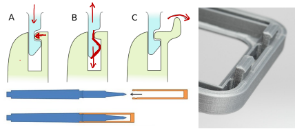
Expansion fit:
If there are large forces/torques acting on these two components so you want them very tight
e.g. you may temporarily expand one component (e.x. with heat) to fit on/around the other, then it will shrink down
Shrink fit:
Same as expansion, but using some cooling process (e.x. liquid nitrogen)
Why do this over heat?
It’s typically more expensive to cool down
The material may deform / weaken – e.g. steel will be degraded if heated up
Transition fit: complete interchangeability is compromised to allow looser tolerance on individual components.
If fit type is not critical.
But even then, why not choose one or the other? Because you don’t want a large gap and the materials/parts cannot withstand the force needed to assemble them with an interference fit.
The pieces are just for alignment – think Ikea assembly pegs; they’re just to align components.
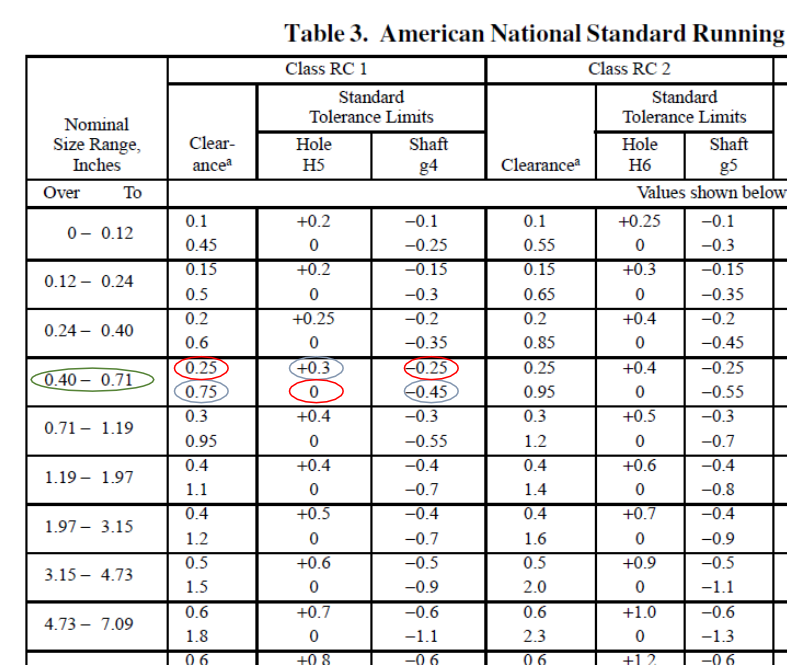
These types are created by ANSI: American National Standards Institute
Exact values are tabulated in many source
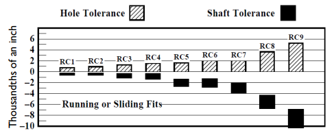
RC: Running and sliding clearance fits
Nine categories:
RC1: Close sliding: assemble without perceptible “play” (e.g. watches)
Less than a 1/1000".
Basically impossible for air, let alone liquids, through.
RC2: Sliding fits: seize with small temperature changes (e.g. )
RC3: Precision running: not suitable for appreciable temperature differences
RC4: Close running: moderate surface speeds and pressures
RC5/6: Medium running: higher speed/pressure
RC7: Free running: where accuracy not essential and/or temperature variations large
RC8/9: Loose running
Go for lower if you want minimal vibration/gaps – no perceivable play.
Has drawbacks:
The less clearance, the easier it is to seize up – especially if two components are touching and made up of different materials (different expansion/contraction rates).
Susceptible to dust, you would have to seal the machine or use it in clean conditions.
If you go less precise, you don’t need to go slow, cheaper operator costs, cheaper tooling
RC Chart
RC Table
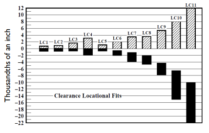
LC: Locational clearance fits
Normally stationary, but freely assembled/disassembled
Used when you need clearance to dis able and clean
LC Chart
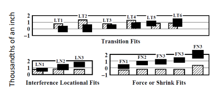
LT: Location transition fits
Accuracy of location important
Small amount of clearance or interference OK
e.g. ikea furniture pegs
LN: Locational interference
When you need friction
Accuracy of location is critical
FN: Force fits
When you need to hold a load (typically uses temporary heating)
Designed to transmit frictional loads from one part to another
Probability density, e.g. given by Gaussian/Normal probability density function: $$p(x) = \frac{1}{\sigma \sqrt{2\pi}}e^{-\frac{(x-x_0)^2}{2\sigma^2}}$$