02-22 Basis #
Change of Basis #
- Previously we’ve seen that a basis for a vector space is a minimal spanning set of vectors.
- We can also define the standard basis vectors, e,x. the standard basis for .$ \mathbb{R}^{3}$ is the set .$\mathbb{E}$:
$$\mathbb{E} = \big(\hat i, \hat j, \hat k \big)$$ $$\dots \equiv ( \vec e_1, \vec e_2, \vec e_3)$$ $$\dots \equiv \left( \begin{bmatrix} 1\\ 0\\ 0\\ \end{bmatrix}, \begin{bmatrix} 0\\ 1\\ 0\\ \end{bmatrix}, \begin{bmatrix} 0\\ 0\\ 1\\ \end{bmatrix}\right) $$
We can represent any set of vectors that form as basis as a linear combination of the standard .$ \mathbb{R}^{3}$ basis vectors
- When you plot a vector, the basis is normally implicit as the standard basis vectors
Change Of Basis Operation: Preserves the geometrical vector but modify its coordinates such that when plotted in the new basis, the original and final vector are physically the same
- Such that we’re essentially re-expressing the coordinates of some .$\vec v$ (formed with basis .$\mathbb{E}$) in some new basis .$\mathbb{E}'$
- We know that the basis vectors define the linear transformation matrix: $$\begin{bmatrix} | & & | \\ \vec e_1 ’ & \dots & \vec e_n ’ \\ | & & | \\ \end{bmatrix}$$
- Thus, we need to solve for the scalars that multiply each of the new basis vectors, .$v_i ’ $, to produce the same physical vector .$\vec v$ as before:
$$\begin{bmatrix} | & | \\ \vec e_1 ’ & \vec e_2 ’ \\ | & | \\ \end{bmatrix}\begin{bmatrix} v_1 ’ \\ v_2 ’ \\ \end{bmatrix} = \begin{bmatrix} v_1 \\ v_2 \\ \end{bmatrix} = \vec v $$
- Generally, we can say that if given a vector .$\vec v$ expressed with coordinates in the standard .$n$-dimensional basis .$\mathbb{E}$, then we can solve for the coordinates .$\vec v ’ $ in a different .$n$-dimensional basis .$A$ with .$\vec v ’ = A^{-1} \vec v$
- .$A$ is formed with the columns of the new basis. To do the opposite (basis .$A \to \mathbb{E}$), we apply .$A$: .$\vec v = A \vec v ’ $
- Finally, suppose that we’re given .$\vec v$ with coordinates in an arbitrary basis .$P$ (matrix with columns .$\vec p_1, \dots, \vec p_n$), and we want to change to another arbitrary basis .$Q$ with columns .$\vec q_1, \dots, \vec q_n$. We must apply the transformation .$Q^{-1} P$. This follows from first transforming .$\vec v$ to the standard basis from .$P$, and then transforming to the new basis .$Q$
- The only question is whether we preserve the coordinates (which are the mathematical representation) and change the physical vector in accordance with the new basis, or preserve the physical vector and find the new coordinates.
- Page 57 has pretty figures
Matrix Change of Basis #
We can apply our knowledge to linear transformations to understand what it means to change the basis of a matrix
- Given transformation .$T \in \mathbb{R}^{n \times n}$ with input .$\vec v_1$ and output .$\vec v_2$, we can apply our column-wise interpretation of the matrix-vector product, but now, we must take care of the fact that our vectors may lie in a different basis than .$E$.
- Suppose we have basis vectors .$\vec a_1, \dots, \vec a_n$ forming .$A \in \mathbb{R}^{n \times n}$, and vectors .$\vec v_1, \vec v_2$ represented in this basis: .$\vec v_i = v_{i,1} ’ \vec a_1 + \dots v_{i,n} ’ \vec a_n$
- Each .$v_{i,k}$ is the .$k$th element of the vector .$\vec v_i$
- We can also represent .$T$ in this basis as .$T ’ $
- We start with .$\vec v_1 = A \vec v_1 ’ $ and .$\vec v_2 = A\vec v_2 ’ $.
- Since .$T\vec v_1 = \vec v_2$ by definition of linear transformation .$T$, we can plug in: .$TA\vec v_1 ’ = A\vec v_2 ’ \Longrightarrow A^{−1} T A \vec v_1 ’ = \vec v_2 ’ $.
- Clearly, just as how we had .$T\vec v_1 = \vec v_2$, we have an analogous transformation in the new basis: .$T ’ \vec v_1 ’ = \vec v_2 ’ $, where .$T ’ = A^{−1} T A $.
.$T ’ $ is equivalent to .$A$, then .$T$, then .$A^{−1}$
Diagonalization #
- Why bother with change of basis? In practical applications, matrix operations form the core of some very computationally heavy algorithms – we need to be able to easily invert matrices, raise them to high powers, and multiply them commutatively; all of these can be accomplished with
diagonal matrices, where all entries not on the diagonal are zero
- An identity matrix of any size, or any multiple of it (a scalar matrix), is a diagonal matrix.
- Its determinant is the product of its diagonal values
- First, we must choose a diagonalizing basis .$A$ that consists of the .$n$ eigenvectors of .$T$.
- This is only possible if .$T$ is diagonalizable, which requires it to have .$n$ linearly independent eigenvectors
- Note this is different from the .$n$ columns being independent!
- Then, to figure out how .$T$ transforms .$\vec v_1$, we write .$\vec v_1 = \vec v_{11} ’ \vec a_1 + \dots + \vec v_{1n} ’ \vec a_n$ $$T \vec v_1 = T \vec v_{11} ’ \vec a_1 + \dots + T v_{1n} ’ \vec a_n$$ $$\dots = v_{11} (T \vec a_1) + \dots + v_{1n} (T\vec a_n)$$ $$\dots = v_{11} (\lambda_1 \vec a_1) + \dots + v_{1n} (\lambda_n \vec a_n)$$
- Using the middle matrix (diagonal!) as a sort of “sifting” matrix; each row only has one nonzero value, so we only multiply the .$v_{1i} \vec a_i$ value by the corresponding .$\lambda_i$: $$T \vec v_1 = \begin{bmatrix} | & & | \\ \vec a_1 & \dots & \vec a_n \\ | & & | \\ \end{bmatrix}\begin{bmatrix} \lambda_{1} & & \\ & \ddots & \\ & & \lambda_{n} \end{bmatrix}\begin{bmatrix} v_1 ’ \\ v_2 ’ \\ \vdots \\ v_n ’ \\ \end{bmatrix}$$
- Notice now we have an equation of the form:
$$T \vec v_1 = AD \vec v_1 ’ \Longrightarrow T\vec v_1 = ADA^{-1} \vec v_1 \Longrightarrow T = ADA^{-1}$$
- Here, .$D$ is the diagonal matrix containing the eigenvalues of the transformation
- One useful result is that .$T^k = AD^k A^{-1}$ (expand and group .$A^{-1}A = I$)
- Since .$D$ is easy to raise to high powers (.$D^k$ contains all diagonal entries raised to the .$k$th power), the computation of numerous transformations becomes much easier
- To raise a diagonal matrix to a power, one can raise each element to that power
- This is only possible if .$T$ is diagonalizable, which requires it to have .$n$ linearly independent eigenvectors
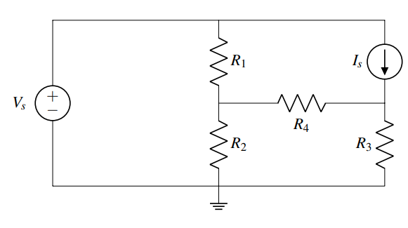
02-24 Intro to Circuit Analysis #
- We will label nodes instead of junctions because all of the junctions that are connected to each other by wires can be labeled with a single voltage variable .$u$.
- A set of such junctions connected to each other only via wires is defined as a node. Nodes have the same voltage at every point on them.
Circuit Analysis Algorithm #
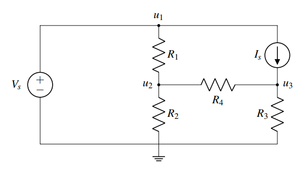
Select a reference ( ground) node .$u_1 = 0$
- This node will have 0 potential – all voltages are measured relative to this node
- Arbitrary selection – any node can be chosen for this purpose.
- In this example, we choose the node at the bottom of the circuit diagram.
Label Nodes .$[u_2, \dots, u_{n}]$
- First lets look at the nodes with voltage set by Voltage Sources. Voltage sources set the voltage of the node they are connected to.
- In the example, there is only one source, .$V_S$, and we label the corresponding source .$u_1$ (names are arbitrary, but must be unique).
- Now we label all remaining nodes in the circuit except the reference – in this example there are two, .$u_2$ and .$u_3$.
Label currents .$[I_1, \dots, I_k]$ through non-wire elements
- The direction is arbitrary (top to bottom, bottom to top, it won’t matter, but stick with your choice in subsequent steps).
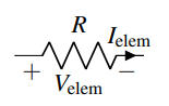
- Then mark the element voltages following the passive sign convention.
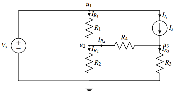
- Label element potentials based on passive sign convention.
- The element voltage for .$I_S$ is not marked in the example since it will not be needed in the calculations below. Same for the voltage source. There is no harm in marking those, too.
- KCL Equations
- Write KCL equations for all nodes with unknown voltage, .$u_2$ and .$u_3$ in the example.
- See Week 2
At .$u_2$ we get (sum of all currents entering the node equals sum of currents exiting): $$I_{R_1} = I_{R_2} + I_{R_4}$$ and similar for .$u_3$: $$I_{R_4} + I_{I_S} = I_{R_3}$$
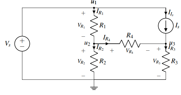
- Element IV Relationships
- Find expressions for all element currents in terms of voltage and element characteristics (e.g. Ohm’s law) for all circuit elements except voltage sources.
- In the example there are five unknown elements: .$R_1, R_2, R_3, R_4, I_S$
- Find expressions for element currents for all elements (except the voltage source) using their characteristics.
- Find expressions for all element currents in terms of voltage and element characteristics (e.g. Ohm’s law) for all circuit elements except voltage sources.
Applying Ohm’s law to the two resistors, we find that
$$I_{R_1} = \frac{V_{R_1}}{R_{1}}$$ $$I_{R_2} = \frac{V_{R_2}}{R_{2}}$$ $$I_{R_3} = \frac{V_{R_3}}{R_{3}}$$ $$I_{R_4} = \frac{V_{R_4}}{R_{4}}$$ $$I_{I_S} = I_S$$ and we have .$u_1 = V_S$
- Solve .$A\vec x = \vec b$ – see
page 12 and/or
slide 14
- .$\vec x = [I_1, \dots, I_k, u_1, \dots, u_n]^T$: The unknown element variables we’re solving for
- .$\vec b \in \mathbb{R}^{k+n}$: The vector of elements values we’re solving for
- Units are either .$V$olts or .$A$mps
- .$A \in \mathbb{R}^{k+n \times k+n}$
- Steps:
- If there are .$n$ nodes (including the ground node), use KCL on .$(n−1)$ nodes to fill in .$(n−1)$ rows of .$A$ and .$\vec b$
- $n-1$ because we know that one of the nodes is ground
- If there .$k$ non-wire elements, use the IV relationships of each non-wire element to fill in the remaining .$k$ equations (rows of .$A$ and values of .$\vec b$).
- If there are .$n$ nodes (including the ground node), use KCL on .$(n−1)$ nodes to fill in .$(n−1)$ rows of .$A$ and .$\vec b$
Branch Current #
- Sometimes we want to solve for branch currents: These are easily obtained from the node voltages and element equations.
For example above, the current .$I_{R_4}$ through resistor .$R_4$ is $$I_{R_4} = \frac{V_{R_4}}{R_4} = \frac{u_2 - u_3}{R_4}$$
Voltage Divider #
Passive sign convention #
- The passive sign convention dictates that positive current should enter the positive terminal and exit the negative terminal of an element.
As long as this convention is followed consistently, it does not matter which direction you arbitrarily assigned each element current to; the voltage referencing will work out to determine the correct final sign. When we discuss power later in the module, you will see why we call this convention “passive.”
Trivial Junctions #
- Trival junction: A junction connecting only two elements.
- KCL dictates that the current entering the junction must be equal to the current exiting. Since there are only two elements, it follows that the two currents must be equal (as long as we label the direction of current flow to be the same – if not, the currents will simply be opposite in sign).
- Therefore, another simplification to our analysis procedure is to label the currents only in the non-wire elements in our circuit (Sometimes these currents are called branch currents)
- When we use KCL, we can now consider nodes (instead of junctions)
- i.e. the current flowing into the node is equal to the current leaving the node.