22.1 Electric Flux #
- Electric Flux: Electric field that passes through a given area
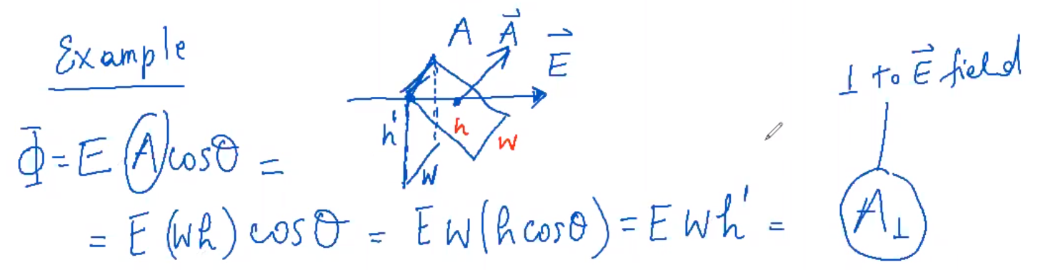
- E.x. for a uniform field .$\vec E$ passing through an area .$A$ at angle .$\theta$ between the field direction and line perpendicular to the area, the flux is defined as
$$\Phi_\vec{E} = \vec E_\perp A = \vec EA_\perp = \vec E A \cos \theta = \vec E \cdot \vec A$$
- E.x. for a uniform field .$\vec E$ passing through an area .$A$ at angle .$\theta$ between the field direction and line perpendicular to the area, the flux is defined as
$$\Phi_\vec{E} = \vec E_\perp A = \vec EA_\perp = \vec E A \cos \theta = \vec E \cdot \vec A$$
- The .$N$umber of field lines passing through unit area perpendicular to the field .$A_\perp$ is proportional to the magnitude of the field .$\vec E$ $$\vec E \propto N/A_\perp \Longrightarrow N \propto \vec EA_\perp = \Phi_\vec{E}$$
- For non-uniform fields:
- We divide up the surface into .$n$ small elements of surface whose areas are .$dA$ where .$dA$ is small enough (1) to be considered flat and (2) so .$E$ varies so little it can considered uniform $$\Phi_\vec{E} = \oint_A \vec E \cdot d\vec A$$
- If .$\Phi > 0$, flux is entering the volume and .$\Phi < 0$ is flux leaving
- Direction:
- For closed surfaces, .$\vec A$ points outwards from the enclosed volume, so flux is positive
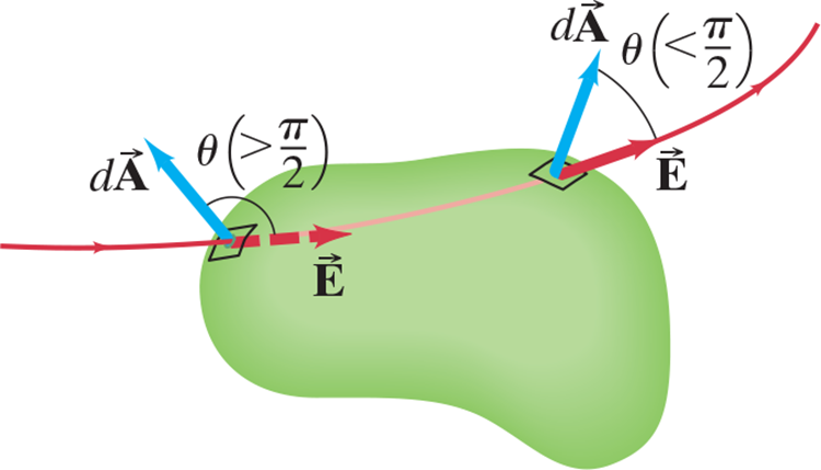
- Further, .$\theta$ (angle between .$d\vec A$ and .$E$) should always be, for electric field…
- Leaving the volume: Less than .$\pi/2$ (so .$\cos\theta > 0$) and .$\Phi > 0$)
- Entering the volume: Greater than .$\pi/2$ (so .$\cos\theta < 0$ and .$\Phi < 0$)
- Net Flux
- In the example above, every line that enters also leaves so .$\Phi = 0$ meaning there is no net flux into or out of the enclosed surface
- Flux will only be nonzero if one of more lines start or end within the surface
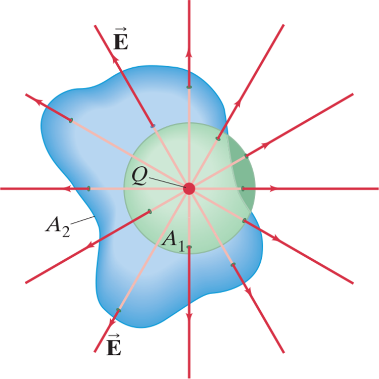
Flux through .$A_1$ is positive, .$A_2$ is negative
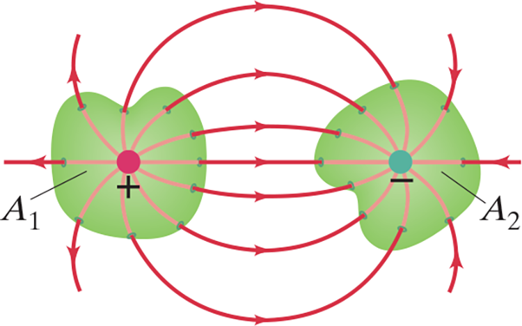
Net flux through .$A$ is negative
22.2 Gauss’s Law #
Gauss’s Law: We can relate flux through a surface and net charge enclosed within said surface by $$\Phi = \oint \vec E \cdot d\vec A = \frac{Q_\text{enclosed}}{\varepsilon_0}$$
- This tells us the difference between the input and output flux of the electric field over any surface is due to charge within that surface.
- This is because we defined .$1 \text{ Coulomb} = \varepsilon_0^{-1} \text{ field lines}$
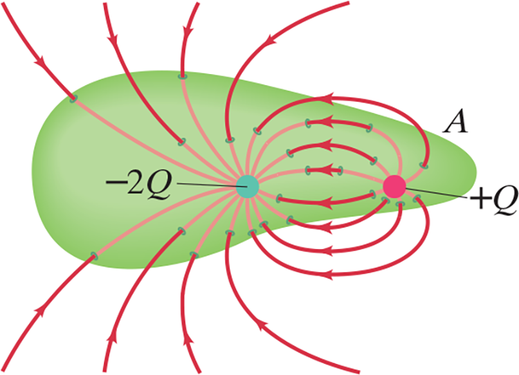
- Notice that it doesn’t matter the distribution of the charge inside the surface
- A charge outside the chosen surface may affect the position of the electric field lines, but it won’t affect the number of lines entering of leaving the surface
Irregular Surfaces:
- Since flux is proportional to the flux lines passing in/out, and the number of lines is the same for .$A_1$ and .$A_2$, so $$\oint_{A_1} \vec E \cdot d \vec A = \oint_{A_2} \vec E \cdot d \vec A = \frac{Q}{\varepsilon_0}$$
- Therefore, this is true for any surface surrounding a single point charge .$Q$
The superposition principle from last chapter also applies to Gauss’s law: The total field .$\vec E$ is equal to the sum of the fields due to each separate charge: $$\oint \vec E_i \cdot d \vec A = \oint \Big(\Sigma \vec E_i \Big) \cdot d \vec A = \sum \frac{Q_i}{\varepsilon_0} = \frac{Q_\text{enclosed}}{\varepsilon_0}$$
22.3 Applications of Gauss’s #
Gauss’s Law to calculate electric fields
- Using symmetry and intuition, draw the electric field lines.
- Enclose all or part of the charge distribution with a Gaussian surface. The electric field should have the same strength at all points on (at least part of) the surface.
- Apply Gauss’s law: .$\Phi_\vec{E} = \oint \vec E \cdot d\vec A = \frac{Q_\text{enclosed}}{\varepsilon_0}$. If .$E$ is constant over (part of) the Gaussian surface, you can pull it outside the integral. This simplification is what allows you to solve for the field.
- Recall .$Q_\text{enclosed} = \frac{\text{(total charge)}}{\text{(total area)}}\times \text{(area enclosed by Gaussian surface)}$
- If you can’t pull .$E$ outside the flux integral, then Gauss’s law don’t work! Use the continuous charge distribution strategy from the prior chapter.
Uniformly Charged Solid Spherical Conductor #
- Charge Outside:
- .$\vec E$ will have the same magnitude at all points along the surface .$A_1$
- Since .$\vec E$ is always orthogonal to the surface, the cosine is always .$1$ $$\Longrightarrow E = \frac{1}{4\pi\varepsilon_0}\frac{Q}{r^2}$$
- We see that the field outside is as if all of the charge was from a single point
- Charge Inside:
- .$\vec E$ will have the same magnitude at all points along the surface .$A_2$
- Thus, .$Q = 0$ because the charge inside the surface .$A_2$ is zero
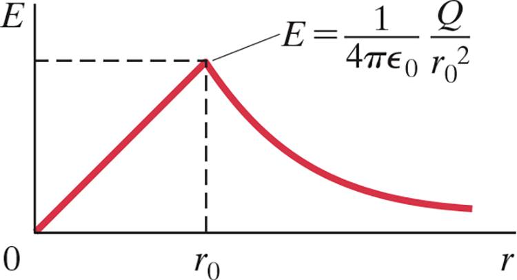
- Hence, .$E = 0$ for .$r < r_0$
- Initial radius is .$r_0$; outside radius is .$r$
- Enclosed charge has charge .$Q$
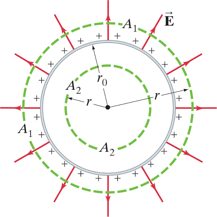
- This result is the same for both hollow and solid spheres because all the charge would lie in a thin layer at the surface.
- If .$Q \neq 0$, current would flow inside the conductor which would build up charge on the exterior of the conductor. This charge would oppose the field, ultimately (in a few nanoseconds for a metal) canceling the field to zero.
Solid Sphere of Charge #
- Charge .$Q$ is distributed uniformly throughout a nonconducting sphere of radius .$r_0$
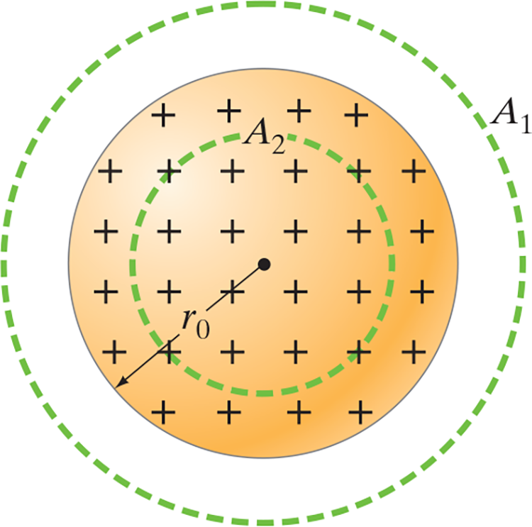
- Charge Outside:
- Same rational as before, $$\oint \vec E \cdot d\vec A = E (4\pi r^2) = \frac{Q}{\varepsilon_0}$$ $$\Longrightarrow E = \frac{1}{4\pi\varepsilon_0}\frac{Q}{r^2}$$
- Again, the field outside is the same as for a point charge in center of sphere
- Charge Inside:
$$\oint \vec E \cdot d\vec A = E (4\pi r^2) = \frac{Q_{\text{enclosed in }A_2}}{\varepsilon_0}$$
- Since .$Q_{\text{enclosed…}} \neq Q$, we define the charge density .$\rho_E$ as the charge per unit volume (.$dQ/dV$) which is constant
- We can then write $$Q_{\text{enclosed}} = Q \cdot \frac{\frac{4}{3}\pi r^3 \rho_E}{\frac{4}{3}\pi r_0^3 \rho_E} = Q\cdot \frac{r^3}{r^3_0}$$ $$ \Longrightarrow E = \frac{1}{4\pi\varepsilon_0}\frac{Q}{r_0^3}r$$ $$$$