Positioning Systems #
Just read Note 21.1-2
Vectors #
Inner Products #
The Euclidean inner product between two vectors $\vec u, \vec v$ is defined as…
$$\langle \vec u, \vec v \rangle \equiv \vec u \cdot \vec v \equiv \vec u^T \vec v$$
$$\dots = \begin{bmatrix} v_1 v_2 \dots v_n \end{bmatrix}\begin{bmatrix} u_1\\ u_2\\ \vdots \\ u_n \end{bmatrix}$$ $$\dots = v_1 u_1 + v_2 u_2 + \dots v_n u_n$$ $$\dots = \sum_{i=1}^n v_i u_i$$
- Naming
- In physics, the inner product is called dot product; $\vec u \cdot \vec v$
- Scalar product is also occasionally used because it produces a scalar output
Properties #
In general, if $\mathbb{V}$ is a real vector space$^{[1]}$, we say that the mapping $\vec u, \vec v \in \mathbb{V} \to \langle \vec u, \vec v \rangle \in \mathbb{R}$ is an inner product iff it satisfies the following properties:
1. Symmetry: $\langle \vec u, \vec v \rangle = \langle \vec v, \vec u \rangle$ for all $\vec u, \vec v \in \mathbb{V}$ #
2. Linearity: #
- Homogeneity: $\langle \gamma \vec u, \vec v \rangle = \gamma \langle \vec u, \vec v \rangle$
- Super position: $\langle \vec u + \vec w, \vec v \rangle = \langle \vec u, \vec v \rangle + \langle \vec w, \vec v \rangle$ for $\vec w \in \mathbb{V}, \gamma \in \mathbb{R}$
3. Positive-definiteness: $\langle \vec v, \vec v \rangle \geq 0$ with equality iff $\vec v = \vec 0$ #
$^{[1]}$In 16A we do not want to think about complex numbers so we tend to have $\vec u, \vec v \in \mathbb{R}^n$
Geometric Interpretation #
The inner product of vectors two vectors is their magnitudes multiplied by the angle between them $$\langle \vec u, \vec v \rangle = \Vert \vec u \Vert \Vert \vec v \Vert \cdot \cos \theta$$
- Proof on page 6
- The inner product does not depend on the coordinate system the vectors are in– it only depends on the relative angle between these vectors and their length.
- Note that we cannot just look at the value of the inner product $\vec u, \vec v$ in making the judgement about the vectors’ similarity, due to the scaling property
- Making the vectors 10 times longer/shorter doesn’t make them any more or less aligned with each other!
- What we can do is normalize the vectors – maintain direction and set magnitude to 1
- E.x. $\hat v = \frac{\vec v}{\Vert \vec v \Vert}$ – the $\hat{ }$ symbol indicates a unit vector (magnitude = 1)
- Nice derivation on page 108
Special Operations #
Motivation: The act of computing an inner product is very simple computationally; it’s just a few additions and multiplications, so computers are highly optimized for computing inner products. Therefore, it is useful to represent other common operations in terms of inner products.
For $\vec v \in \mathbb{R}^n$
- Sum of Components: $\langle \vec 1, \vec v \rangle = v_0 + v_1 + \dots + v_n$
- Average: $\langle \hat n^{-1}, \vec v \rangle = \frac{v_0}{\hat n} + \frac{v_1}{\hat n} + \dots + \frac{v_n}{\hat n} = \frac{v_0 + \dots + v_n}{n}$
- Sum of Squares: $\langle \vec v, \vec v \rangle = v_0^2 + v_1^2 + \dots + v_n^2$
- Selective Sum: $\langle \vec e_2 + \vec e_5 + \dots + e_n, \vec v \rangle = v_2 + v_5 + \dots v_n$
Orthogonal Vectors #
Two vectors $\vec v, \vec u \in \mathbb{R}^n$ are orthogonal if their inner product is zero, i.e. $\langle \vec v, \vec u \rangle = 0$
- Orthogonality can be thought of perpendicularity to higher dimensions than two/three
- Note that the standard unit vectors are always orthogonal to each other.
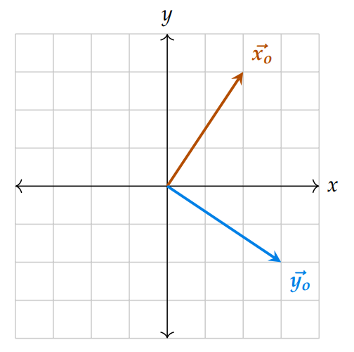
- E.x. orthogonal vectors in $\mathbb{R}^2$ to the right:
Norms #
The Euclidean Norm (or 2-norm) of a vector represents the vector’s length, or magnitude. Defined as $\Vert \vec v \Vert = \sqrt{v_1^2 + \dots v_n^2} = \sqrt{\langle \vec v, \vec v \rangle}$ where the inner product on the right is the Euclidean inner product
- The norm of a vector is the magnitude
- This corresponds to the usual notion of distance in $\mathbb{R}^2, \mathbb{R}^3$
- The set of points with equal Euclidean norm is a circle in $\mathbb{R}^2$ or a sphere in $\mathbb{R}^3$
- Aside: More generally, any choice of inner product will give rise to a corresponding norm via defining $\Vert \vec v \Vert := \sqrt{ \langle \vec v, \vec v \rangle}$
Properties #
For $\vec v, u \in \mathbb{R}^2$…
1. Non-negativity: $\Vert \vec v \Vert \geq 0$ #
2. Zero Vector: $\Vert \vec v \Vert = 0 \iff \vec v = \vec 0$ #
3. Scalar Multiplication: $\Vert \gamma \vec v \Vert = \vert \gamma \vert \Vert \vec v \Vert$ #
4. Triangle Inequality: $\Vert \vec v + \vec u \Vert \leq \Vert \vec v \Vert + \Vert \vec u \Vert$ #
Cauchy-Schwarz Inequality #
$$\vert \langle \vec v, \vec u \rangle \vert \leq \Vert \vec v \Vert \Vert \vec u \Vert$$
We can prove this knowing $\vert \cos \theta \vert \leq 1$:
$$\vert \langle \vec v, \vec u \rangle \vert = \big\vert \Vert \vec u \Vert \Vert \vec u \Vert \cdot \cos \theta \big\vert $$ $$\vert \langle \vec v, \vec u \rangle \vert = \Vert \vec u \Vert \Vert \vec u \Vert \cdot \big\vert\cos \theta \big\vert $$ $$\therefore \vert \langle \vec v, \vec u \rangle \vert \leq \Vert \vec u \Vert \Vert \vec u \Vert $$
Projections #
- The vector projection of $\vec x$ onto $\vec y$ — $\text{proj}_{\vec y}\vec x$ — refers to the component of $\vec x$ that is aligned in the same direction as $\vec y$– or exactly opposite; it helps to imagine a line going through $\vec y$
- By definition, we see that $\text{proj}_{\vec y}\vec x \in \text{Span} \{\vec y \}$
- If the projection is zero, then the vectors are orthogonal – there is no component of $\vec y$ that is aligned with $\vec x$
- We can break up $\vec x$ into it’s parallel and perpendicular components to $\vec y$, $\vec x_\parallel, \vec x_\perp$
- The length of the parallel component $\Vert \vec x_\parallel \Vert$ gives the scalar projection of $\vec x$ onto $\vec y$ $$\cos \theta = \frac{\langle \vec x, \vec y \rangle}{\Vert \vec x \Vert \Vert \vec y \Vert}$$ $$\therefore \text{comp}_{\vec{y}} \vec x = \Vert \vec x_\parallel \Vert = \cos\theta \Vert \vec x \Vert$$ $$\dots = \frac{\langle \vec x, \vec y\rangle}{\Vert \vec y \Vert} $$
- This is the scalar projection, which we can give direction by multiplying it by $\hat y$
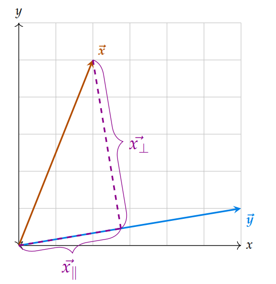
- This new, unique vector is closest to $\vec x$ as measured by the norm – page 9
- The above only uses generic properties of the inner product, and does not need to the specific choice of the Euclidean inner product to work out.
- See also: Math 53 12.3: Projections
Trilateration #
- We know the locations of the beacons $\vec a_1,\vec a_2,\vec a_3$
- We know the distances $d_1,d_2,d_3$
- We want to find the position of $\vec x$
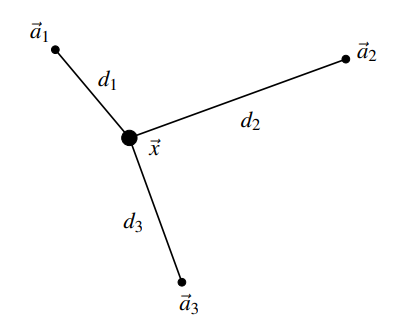
- These two equations are linear in $\vec x$, so we can then stick them into a matrix
- This system can be solved for a location
- Notice that three circles uniquely define a point in 2D; this argument extends in 3D to four spheres, 4D to five hyper-spheres, etc.
$$\Vert \vec x - \vec a_1 \Vert^2 = d_1^2$$ $$\Vert \vec x - \vec a_2 \Vert^2 = d_2^2$$ $$\Vert \vec x - \vec a_3 \Vert^2 = d_3^2$$ $$\equiv$$ $$(\vec x - \vec a_i)^T (\vec x - \vec a_i) = d_i^2$$ $$\equiv$$ $$\vec x^T \vec x - \vec x^T\vec a_i -\vec a_i^T\vec x + \vec a_i^T \vec a_i - = d_i^2$$ $$\equiv$$ $$\Vert \vec x \Vert^2 - 2 \langle \vec x, \vec a_i \rangle + \Vert \vec a_i \Vert^2 = d_i^2$$
We have squared terms (not linear!) involving unknown variable $\vec x$
We’ll subtract equation 1 from equation 2, and separately again from equation 3. $$2 (\vec a_1 - \vec a_2)^T \vec x = \Vert \vec a_1 \Vert^2 - \Vert \vec a_2 \Vert^2 - d_1^2 + d_2^2$$ $$2 (\vec a_1 - \vec a_3)^T \vec x = \Vert \vec a_1 \Vert^2 - \Vert \vec a_3 \Vert^2 - d_1^2 + d_3^2$$ $$\equiv$$ $$\begin{bmatrix} 2 (\vec a_1 - \vec a_2)^T \\ 2 (\vec a_1 - \vec a_3)^T \\ \end{bmatrix}\vec x = \begin{bmatrix} \Vert \vec a_1 \Vert^2 - \Vert \vec a_2 \Vert^2 - d_1^2 + d_2^2 \\ \Vert \vec a_1 \Vert^2 - \Vert \vec a_3 \Vert^2 - d_1^2 + d_3^2 \\ \end{bmatrix}$$
Signals #
Signal: a message that contains information as a function of, in this class, time – can also be a function of space (i.e. an image)
- Discrete-time Signal: defined at specific points in time (for example, every minute) – can represent as a list of numbers
- Continuous-Time Signal: defined over all time – not focused on in 16A
- We can represent a discrete-time signal as a list of numbers, and thus as a vector where each element is the value at a single time point
Every element of the vector represents the signal value at one timestep. We’ll use the notation $s[k]$ to represent the $k$-th element of the vector where initial element is at $k = 0$. E.x. in the signal $\vec s$ above, $s[0] = 0$, $s[1] = 1$, etc.
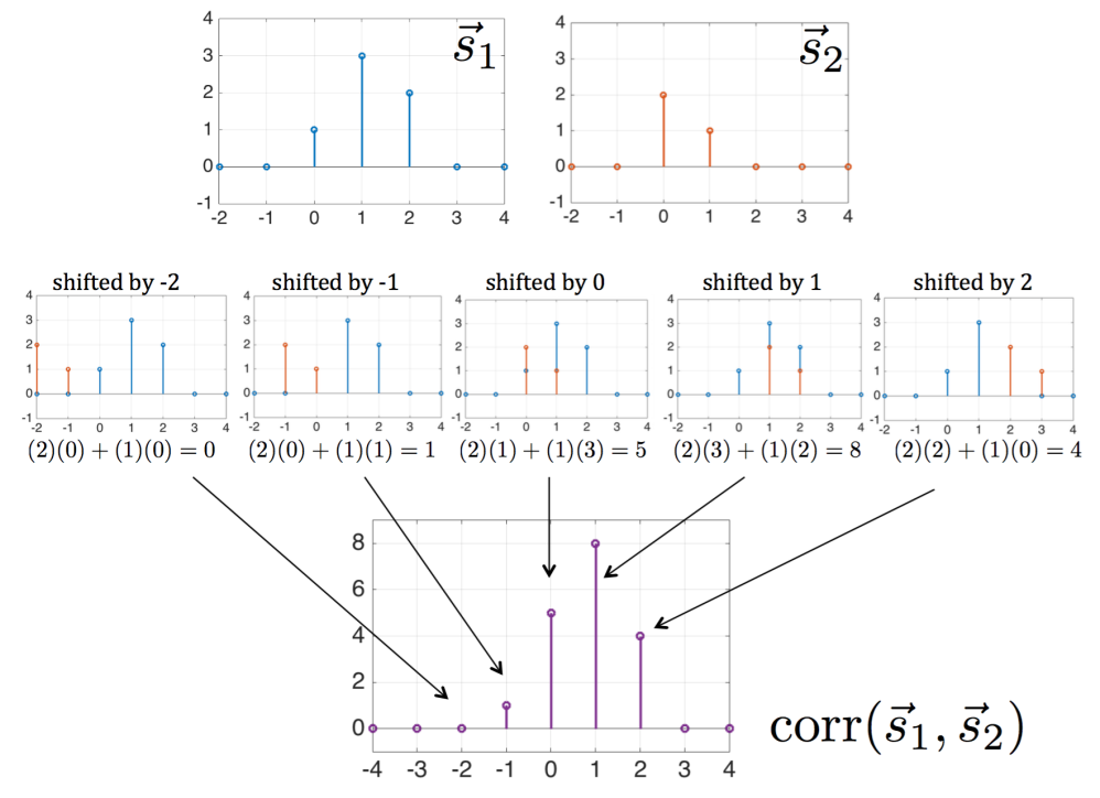
Cross-Correlation #
Cross-correlation: Measure of the similarity between two signals $\vec x$ and $\vec y$ based on the inner product.
$$\text{corr}_{\vec x} ( \vec y) [k] = \sum^{\infty}_{i=-\infty} x[i] y[i−k]$$ $$\dots = \left\langle \vec x, \vec y^{(k)} \right\rangle$$
- $\vec x, \vec y$: input signals
- $\text{corr} _{\vec x} ( \vec y) [k]$: $k$-th element of their cross-correlation
- We typically iterate over $[-l, L+l]$
- $L, l$ The larger and smaller signal lengths, respectively
- $x[n], y[n] = 0$ for any $n$ that they are not defined for
- When the inner product is large, $\vec x, \vec y$ are more similar, and when it’s small, they are more different.
- The cross-correlation checks the inner product at all relative shifts between the signals, so it tells us how similar two signals are at every shift.
- Autocorrelation: a correlation between a signal and itself
- Tells us how similar a signal is to all shifts of itself.
- Not commutative: $\text{corr}_{\vec x} ( \vec y) \neq \text{corr}_{\vec y} ( \vec x)$
- Aside: convolution is an operation similar to correlation but commutative
- Aside: Circular Correlation
- E.x. for $\vec s_1 = \begin{bmatrix}1 \ 3 \ 2\end{bmatrix}^T$, $\vec s_2 = \begin{bmatrix}2 \ 1\end{bmatrix}^T$:
- $\text{corr}_{\vec s_1} ( \vec s_2) [0] = (1)(2) + (3)(1) + (2)(0) = 5$
- Using numpy:
numpy.correlate([1, 3, 2], [2, 1], ‘full’)