28.1 Magnetic Field Due to a Straight Wire #
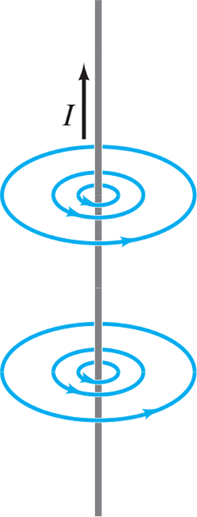
- Magnetic fields due to the electric current in a long straight wire forms circles with the wire at the center
- This field is proportional directly with current .$I$ and inversely with distance .$r$:
$$B = \frac{\mu_0}{2\pi} \cdot \frac{I}{r}$$
- .$\mu_0 = 4\pi \times 10^{-7} \text{ T$\cdot$m/A}$ is the permeability of free space
28.2 Force between Two Parallel Wires #
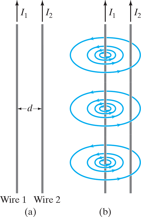
- Since current-carrying wires feel a force in magnetic fields, and because current-carrying wires emit magnetic fields, current-carrying wires exert a force on one another
- Magnetic field .$B_1$ produced by .$I_1$ is given by $$B_1 = \frac{\mu_0}{2\pi} \cdot \frac{I_1}{d}$$
- Parallel currents in the same direction attract while antiparallel repel
- Using .$F = IlB$ we can write the force .$F_2$ exerted by .$B_1$ on length .$l_2$ carrying .$I_2$ has magnitude:
$$F_2 = I_2 l_2 B_1$$
- Notice that the force on .$I_1$ is due to the field produced by .$I_1$
- Thus, subbing .$B_1$ into the .$F_2$ formula we find the force on length .$l_2$: $$F_2 = \frac{\mu_0}{2\pi} \cdot \frac{I_1 I_2}{d}l_2$$
28.3 Definitions of the Ampere and the Coulomb #
One ampere can be defined as that current flowing in each of two long parallel wires exactly 1 m apart, which results in a force of exactly .$2\times10^{-7}$ N per meter of length of each wire
- This was the standard we used prior because it is readily reproducible (that is, it’s called an operational definition)
- Coulomb is defined in terms of the ampere being exactly one ampere-second: .$\text{1 C = A $\cdot$ s}$
- Now we define an ampere ampere by saying it’s .$\text{1 C = A $\cdot$ s}$ and we know the Coulomb because it’s mutually assigned the exact value .$e = 1.60176636 \times 10^{-19}\text{ C}$
28.4 Ampère’s Law #
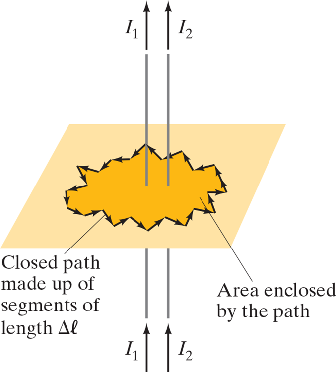
- If we don’t have a straight line, we use ampere’s law given below
- We take a infinite tiny segments and dot it with the field at the segment: $$\oint \vec B \cdot d \vec l = \mu_0 I_\text{encl}$$
- Note that .$\vec B$ in Ampere’s law isn’t necessarily due only to the current .$I_\text{encl}$
- As with Gauss’s law for the electric field, Ampere’s law practical value to calculate the magnetic field is limited, however, mainly to simple or symmetric situations.
- Its importance is that it relates the magnetic field to the current in a direct and mathematically elegant way.
- Ampère’s law is considered one of the basic laws of electricity and magnetism: It is valid for any situation where the currents and fields are steady and not changing in time, and no magnetic materials are present
Problem Solving: #
- Ampère’s law, like Gauss’s law, is always a valid statement. But as a calculation tool it is limited mainly to systems with a high degree of symmetry. The first step in applying Ampère’s law is to identify useful symmetry.
- Choose an integration path that reflects the symmetry. Search for paths where .$\vec B$ has constant magnitude along the entire path or along segments of the path. Make sure your integration path passes through the point where you wish to evaluate the magnetic field.
- Use symmetry to determine the direction of .$\vec B$ along the integration path. With a smart choice of path, .$\vec B$ will be either parallel or perpendicular to the path.
- Determine the enclosed current, .$I_\text{encl}$. Be careful with signs. Let the fingers of your right hand curl along the direction of .$\vec B$ so that your thumb shows the direction of positive current. If you have a solid conductor and your integration path does not enclose the full current, you can use the current density (current per unit area) multiplied by the enclosed area.
28.5 Magnetic Field of a Solenoid and a Toroid #
- Solenoid: A long looping coil of wire carrying a dc current
- The current in each loop produces a magnetic field
- The total magnetic field is the sum of the fields due to each loop
- Direction is determined by the right hand rule $$\oint \vec B \cdot d \vec l = \mu_0 NI$$
Magnetic field due to a solenoid
(a) a few loosely spaced loops; (b) for many closely spaced loops, the field is nearly uniform.
Cross-sectional view into a solenoid.
The magnetic field inside is straight except at the ends. Red dashed lines indicate the path chosen for use in Ampère’s law. .$\odot$ and .$\otimes$ are electric current direction (in the wire loops) out of the page and into the page.
$$\int_c^d \vec B \cdot d \vec l = Bl_{cd}$$
- With .$n = N/l$ is number of loops per unit length we can simplify to $$B = \mu_0 nI$$
- Now, we see that the field does not depend on position within the solenoid, so .$\vec B$ is uniform.
- This is strictly true only for an infinite solenoid, but it is a good approximation for tightly wound real ones for points not close to the ends.
28.6 Biot-Savart Law #
- A current .$I$ flowing in any path can be considered as many tiny current elements, such as .$d \vec l$
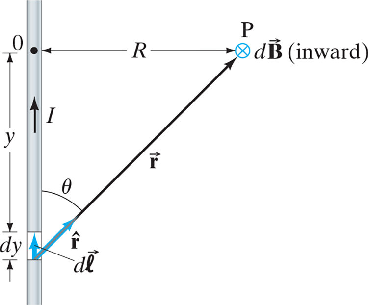
- Then, .$d\vec B$ at any point .$P$ in space due to this element of current is given by Biot-Savart law: $$d\vec B = \frac{\mu_0 I}{4\pi} \frac{d\vec l \times \hat r}{r^2} = \frac{\mu_0 I}{4\pi} \frac{dl \sin\theta}{r^2}$$
- .$\vec r$ is the displacement vector from the element .$d \vec l$ to the point .$P$
- .$\hat r$ is the unit vector in the direction .$\vec r$
- .$\theta$ is the angle between .$d\vec l$ and .$\vec r$
Biot-Savart Law
The field at P due to current element .$I d\vec l$ is .$d \vec B = (\mu_0 I/4\pi)(d\vec l \times \hat r/r^2)$
- An important difference between the Biot-Savart law and Ampère’s law is that the later, .$\oint \vec B \cdot d\vec l = \mu_0 I_\text{encl}$, .$\vec B$ is not necessarily due only to the current enclosed by the path of integration.
- But in the Biot-Savart law the field .$d\vec B$ is due only, and entirely, to the current element .$I d\vec l$ – that is, to find the total .$\vec B$ at any point in space, it is necessary to include all currents.
Biot-Savart strategy for finding a magnetic field
- Select some tiny piece of wire .$d \vec l$ and draw the vector .$\vec r$ pointing from said piece to the location at which you’re finding the magnetic field
- Using Biot-Savart, calculate the magnitude and direction of the infinitesimal magnetic field .$d\vec B$ generated by that piece
- Add up all those magnetic field contributions by integrating over the wire, using vector components if needed.
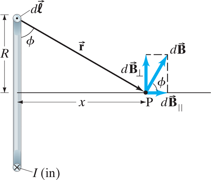
Straight Wire #
$$B = \frac{\mu_0 I}{4\pi}\int_{y =-\infty}^{+\infty} \frac{dy \sin\theta}{r^2}$$
$$dy = dl; r^2 = R^2 + y^2$$
$$dy = \dots = \frac{r^2 d\theta}{R}$$
$$B = \frac{\mu_0 I}{4\pi}\frac{1}{R}\cdot \bigg[-\cos\theta\bigg]_{\theta = 0}^\pi $$
$$\dots = B = \frac{\mu_0 I}{2\pi R}$$
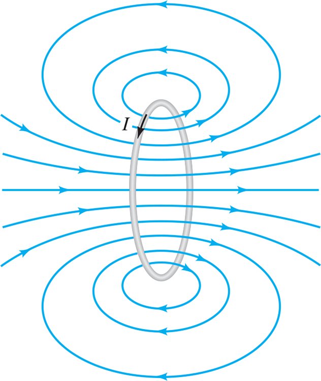
Current Loop #
$$dB = \frac{\mu_0 I dl}{4\pi r^2}$$
$$d\vec l \perp \vec r; \vert d\vec l \times \hat r \vert = dl$$
$$B = \int dB \cos \phi = \int dB \frac{R}{r}$$
$$\dots = \int dB \frac{R}{(R^2 + x^2)^{\frac{1}{2}}}$$
$$\dots = \frac{\mu_0 I}{4\pi}\frac{R}{(R^2 + x^2)^{\frac{3}{2}}} \bigg[L\bigg]_{L = 2\pi R}$$
$$\dots = \frac{\mu_0 I}{2R}$$
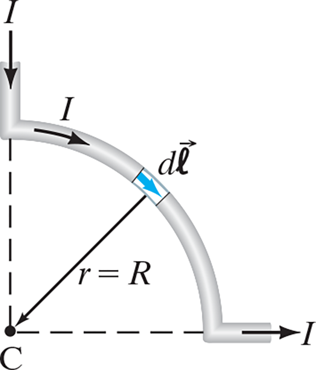
Quarter Wire Segment #
$$dB = \frac{\mu_0 I}{4\pi}dl$$ $$B = \frac{\mu_0 I}{4\pi} \bigg[L\bigg]_{L =\frac{1}{4}\cdot 2\pi R}$$ $$\dots = \frac{\mu_0 I}{8 R}$$
28.6.1 Magnetic Dipole Field #
- Recall that a magnetic dipole is .$\mu = NIA$ (number of loops, current, and area of coil)
- The magnetic field produced by magnetic dipoles is $$B = \frac{\mu_0 IR^2}{2(R^2 + x^2)^{\frac{3}{2}}}$$
- This can be written in tirms of the magnetic dipole .$\mu = IA = I\pi R^2$ for one loop: $$B = \frac{\mu_0}{2\pi} \frac{\mu}{(R^2 +x^2)^{\frac{3}{2}}}$$ and at distances far from the loop .$x \gg R$ this becomes $$B \approx \frac{\mu_0}{2\pi} \frac{\mu}{x^3}$$
28.7 Magnetic Field Due to a Single Moving Charge #
- Realize that Biot-Savart works only when considering constant currents that do not change in time significantly over a significant length of wire
- Additionally, the law is difficult to confirm experimentally:
- Particles would shoot out of the field before they (and thus the field) could be measured for any significant .$B$.
- If .$v$ is slow enough to be measured, .$B$ is small enough it’s going to be drowned out by experimental noise
- From the particles frame, it’s at rest (not moving wrt itself). And since it’s at rest, it shouldn’t create a field. However, it’s moving because it’s creating a field!
- Einstein explains this with special relativity
- Observers in two different reference frames, moving relative to each other, will not observe the same .$\vec E$ and .$\vec B$ fields
- Particles would shoot out of the field before they (and thus the field) could be measured for any significant .$B$.
What see from the perspective other than the particle: The magnetic field at one single instant due to a single positive charge .$q$ moving at velocity .$\vec v$.
28.8 Magnetic Materials—Ferromagnetism (not covered) #
- Magnetic fields are produced by (1) magnets and (2) electric currents
- Ferromagnetism: Materials that are magnetic
- At a small enough resolution (less than 1mm areas!), domains exist which behave like tiny magnets – they have two poles
- The more domains that are aligned in one direction, the stronger the magnetic field
- These domains can be moved around (through dropping or hammering the magnet)
- Heating also reduces magnetism – increasing temp increases the random thermal motion of atoms
- Above the Curie Temperature (1043K for iron), a magnet cannot be made at all
- As a consequence, at lower temperatures, some materials are magnetic
(a) An unmagnetized piece of iron is made up of domains that are randomly arranged. Each domain is like a tiny magnet; the arrows represent the magnetization direction, with the arrowhead being the N pole. (b) In a magnet, the domains are preferentially aligned in one direction (down in this case), and may be altered in size by the magnetization process.
- Today, we believe that all magnetic fields come from electric currents
- Electrons produce a (tiny) magnetic field, as if they and their electric charges were spinning about their own additional axes
- Realize that while .$\vec B$ lines form closed loops, .$\vec E$ lines go from a positive to negative electron
28.9 Electromagnets and Solenoids—Applications (not covered) #
Solenoids act like magnets; they have poles (determined by the right hand rule)
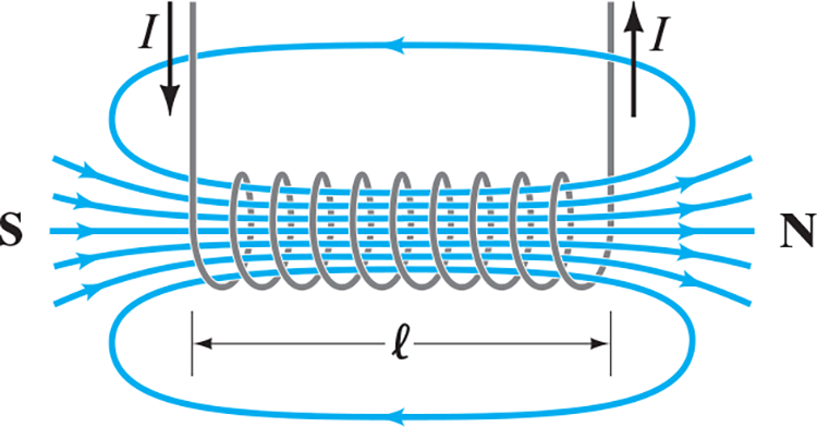 Magnetic field of a solenoid. The north pole of this solenoid, thought of as a magnet, is on the right, and the south pole is on the left.
If a piece of iron is placed inside a solenoid, the magnetic field is increased greatly
- The domains of the iron are aligned by the magnetic field produced by the current; that is, the iron becomes a magnet. This system of the iron-core solenoid is called an electromagnet
- The resulting magnetic field is the sum of the field due to the solenoid’s current and the field due to the iron, and can be hundreds or thousands of times larger than the field due to the current alone
- The alloys of iron used in electromagnets acquire and lose their magnetism quite readily when the current is turned on or off, and so are referred to as “soft iron.” (It is “soft” only in a magnetic sense.)
- Soft iron is usually used in electromagnets so that the field can be turned on and off readily.
- Iron that holds its magnetism even when there is no externally applied field is called “hard iron.”
- Hard iron is used in permanent magnets.
- Whether iron is hard or soft depends on heat treatment, type of alloy, and other factors.
- Sometimes an iron core is not present—the magnetic field then comes only from the current in the wire loops.
- A large field .$B$ in this case requires a large current .$I$ which produces a large amount of waste heat since .$P = I^2 R$.
- But if the current-carrying wires are made of superconducting material kept below the transition temperature then very high magnetic fields can be produced, and no electric power is needed to maintain the large current in the superconducting coils.
- Note that energy is required to refrigerate the coils at the low temperatures where they superconduct.
28.10 Magnetic Fields in Magnetic Materials; Hysteresis (not covered) #
- The solenoid field is produced just .$n$ loops per unit length is .$B_0 = \mu_0 n I$
- If a solenoid contains a ferromagnetic material (e.x. iron), then we need to consider it’s field .$B_M$ produced in our total field calculation:
$$\vec B = \vec B_0 + \vec B_M$$
- Often, .$B_M \gg B_0$
- We can also write this equation as
$$B = \mu n I$$
- .$\mu$ is the magnetic permeability (not electric dipole moment!)
- However, while .$\mu$ is a characteristic of the material, it is not constant for ferromagnetic materials; rather, it depends on the value of the “external field” .$B_0$
- .$\mu \gg \mu_0$ for ferromagnetic materials