The content of these notes are solid, but formatting is not since they’re exported from Notion.
Unit 1: Exploring One-Variable Data #
Types of Variables #
- Categorical variables assigns labels that place each individual into a particular group, called a category.
- Zip code. hair color
- Quantitative variables takes number values that are quantities—counts or measurements.
- Height, GPA
- Explanatory
- x on graph
- independent variable — what we’re changing
- measures an outcome of a study.
- Response
- y on graph
- (potentially) dependent variable — what we’re measuring
- may help predict or explain changes in a response variable
- Confounding
- Any factor that messes skews data
- Confounding occurs when two variables are associated in such a way that their effects on a response variable cannot be distinguished from each other.
- If you are asked to identify a possible confounding variable in a given setting, you are expected to explain how the variable you choose (1) is associated with the explanatory variable and (2) is associated with the response variable.
Frequencies #
- A frequency table shows the number of individuals having each value.
- A relative frequency table shows the proportion or percent of individuals having each value.
- A marginal relative frequency gives the percent or proportion of individuals that have a specific value for one Categorical variable.
- What percent of people in the sample are environmental club members?
- What proportion of people in the sample never used a snowmobile?
- What percent of people in the sample are environmental club members?
- A joint relative frequency gives the percent or proportion of individuals that have a specific value for one Categorical variable and a specific value for another Categorical variable.
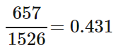
- We can compute marginal relative frequencies for the row totals to give the distribution of snowmobile use for all the individuals in the sample:
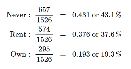
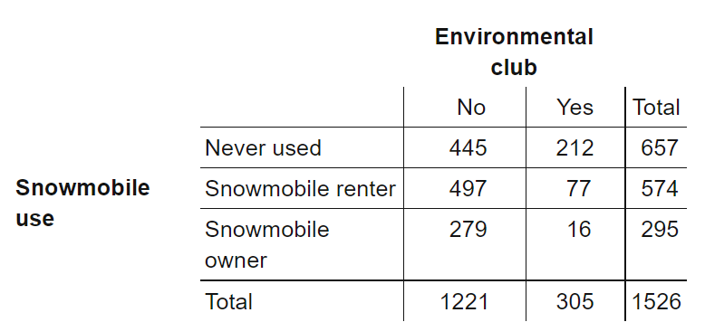
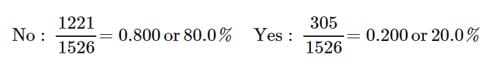
- We can compute marginal relative frequencies for the column totals to give the distribution of environmental club membership in the entire sample of 1526 park visitors
- We can compute marginal relative frequencies for the row totals to give the distribution of snowmobile use for all the individuals in the sample:
- A conditional relative frequency gives the percent or proportion of individuals that have a specific value for one Categorical variable among individuals who share the same value of another Categorical variable (the condition).
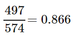
- What proportion of snowmobile renters in the sample are not environmental club members?
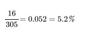
- What percent of environmental club members in the sample are snowmobile owners?
- What proportion of snowmobile renters in the sample are not environmental club members?
Types of Graphs #
- Pie Chart — Categorical
- Need frequency value and corresponding label
- Doesn’t show sample size
- Need frequency value and corresponding label
- Bar Graph — Categorical
- Needs bar labels, axis names, units, vertical axis scale should start at 0
- A side-by-side bar graph displays the distribution of a Categorical variable for each value of another Categorical variable. The bars are grouped together based on the values of one of the Categorical variables and placed side by side.
- A segmented bar graph displays the distribution of a Categorical variable as segments of a rectangle, with the area of each segment proportional to the percent of individuals in the corresponding category.
- Doesn’t show sample size, only proportions
- This can be fixed by using a mosaic plot which scales the width corresponding to size
- Doesn’t show sample size, only proportions
- Dotplot — Quantitative
- A dot plot shows each data value as a dot above its location on a number line.
- Needs title, axis label, unit of measurement
- How to find percentile
- Percentile is the percent of people you’re better than, or percent of people that are worse than you
- Find how many points the decided point is ahead of, then divide by sample size
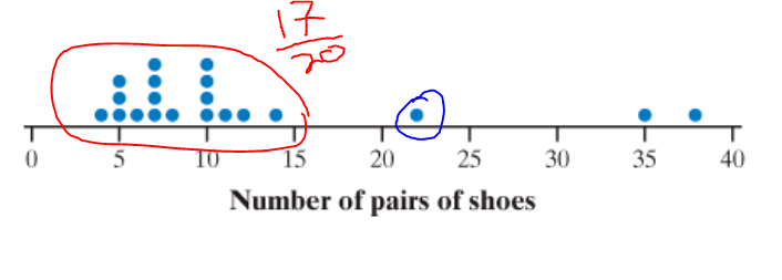 The blue point is greater than 17 points, making it 17/20 —> in the 85% percentile
- Stemplot — Quantitative
- A stemplot shows each data value separated into two parts: a stem, which consists of all but the final digit, and a leaf, the final digit. The stems are ordered from lowest to highest and arranged in a vertical column. The leaves are arranged in increasing order out from the appropriate stems.
- Needs key and title
- Key should give context
Key: 8|2 is a [context — student whose resting pulse rate] is 82 [beats per minute]
- Histogram — Quantitative
- A histogram shows each interval of values as a bar. The heights of the bars show the frequencies or relative frequencies of values in each interval.
- Needs title, axis label, unit of measurement
- Boxplot — Quantitative
Describing Distributions (SOCS) + Context #
Always be sure to include context when you are asked to describe a distribution. This means using the variable name, not just the units the variable is measured in. When comparing distributions of Quantitative data, it’s not enough just to list values for the center and variability of each distribution. You have to explicitly compare these values, using words like “greater than,” “less than,” or “about the same as.”
Shape (Skew) #
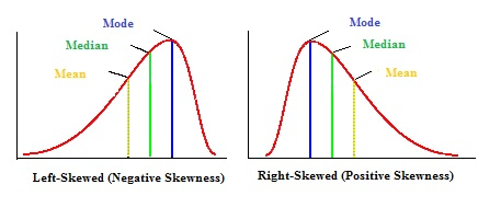
- A distribution is skewed to the right if the right side of the graph is much longer than the left side.
- A distribution is skewed to the left if the left side of the graph is much longer than the right side.
The distribution of [context] is [skewed left/right/sym]
Outlier #
- Gaps too
- Low outliers < Q1 − 1.5 × IQR
- High outliers > Q3 + 1.5 × IQR
- Doesn’t follow trend, large residual
The [context — games played with 5 points / person with a height of 3’] appears to be an outlier
Center #
- Mean / average
- The mean is sensitive to extreme values in a distribution.
- These may be outliers, but a skewed distribution that has no outliers will also pull the mean toward its long tail.
- We say that the mean is not a resistant measure of center — Shouldn’t be used with skew or outliers
- The mean is sensitive to extreme values in a distribution.
- Median
- Resistant — should be used with outliers and skew
Spread / Variability #
- Range
- Not resistant — Shouldn’t be used with skew or outliers
The data vary from [min] to [max] [context — points scored / heights] meaning it had a range of [max - min]
- Standard Deviation
- Measure of the typical distance of the values in a distribution from the mean.
- It should be used only when the mean is chosen as the measure of center.
- sx is not a resistant measure of variability — Shouldn’t be used with skew or outliers
- Larger values of sx indicate greater variation
- sx is always greater than or equal to
- The Interquartile Range (IQR)
- What
- The quartiles of a distribution divide the ordered data set into four groups having roughly the same number of values. To find the quartiles, arrange the data values from smallest to largest and find the median.
- The first quartile Q1 is the median of the data values that are to the left of the median in the ordered list.
- The third quartile Q3 is the median of the data values that are to the right of the median in the ordered list.
- IQR = Q3 - Q1
- Resistant because they are not affected by a few extreme value — should be used with outliers
- What
Why is it important? #
- They might be inaccurate data values. Maybe someone recorded a value as 10.1 instead of 101. Perhaps a measuring device broke down. Or maybe someone gave a silly response, like the student in a class survey who claimed to study 30,000 minutes per night! Try to correct errors like these if possible. If you can’t, give summary statistics with and without the outlier.
- They can indicate a remarkable occurrence. For example, in a graph of net worth, Bill Gates is likely to be an outlier.
- They can heavily influence the values of some summary statistics, like the mean, range, and standard deviation.
- It can make it easier to see associations between variables
- An association exists when there is a difference in outcome for different inputs
- We can only find definitive associations for the sample, and we have to use test to find out if we can extrapolate this data to a larger sample
- For example, there may be an association between AP Stats students and not having post-HS plans and overall being less likely to go to University when compared to AP Calc students
Five number summary (+ boxplot) #
- Min
- Q1
- Median
- Q3
- Max
Standardized score (z-score) — the ’test statistic' #
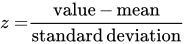
Tells us how many standard deviations from the mean the value falls, and in what direction.
Values larger than the mean have positive z-scores. Values smaller than the mean have negative z-scores.
Shape must be close to normal for z-scores to work
- Never say that a distribution of Quantitative data is Normal. Real-world data always show at least slight departures from a Normal distribution. The most you can say is that the distribution is “approximately Normal.”
- 68–95–99.7
- Approximately 68% of the observations fall within σ of the mean μ
- Approximately 95% of the observations fall within σ 2 of the mean μ
- Approximately 99.7% of the observations fall within σ 3 of the mean μ
Transforming Data #
- Multiplying / dividing by a constant (Units converted)
- Multiplies (divides) center and location (mean, five-number summary, percentiles) by b
- Multiplies (divides) measures of variability (range, IQR, standard deviation) by b
- Does not change the shape of the distribution
- Adding/subtracting constant
- Adds a to (subtracts a from) measures of center and location (mean, five-number summary, percentiles)
- Does not change measures of variability (range, IQR, standard deviation)
- Does not change the shape of the distribution
Percentile #
invNorm(.9, 0, 1)would find the z-score of 90%- Good video
Unit 2: Exploring Two-Variable Data #
How to Describe a Scatterplot #
- Use CONTEXT
- Direction (association)
- Two variables have a positive association when above-average values of one variable tend to accompany above-average values of the other variable and when below-average values also tend to occur together.
- More [x-unit], more [y-unit]
- Two variables have a negative association when above-average values of one variable tend to accompany below-average values of the other variable.
- More [x-unit], less [y-unit]
- There is no association between two variables if knowing the value of one variable does not help us predict the value of the other variable.
Form: #
- A scatterplot can show a linear form or a nonlinear form.
- The form is linear if the overall pattern follows a straight line.
- Otherwise, the form is nonlinear.
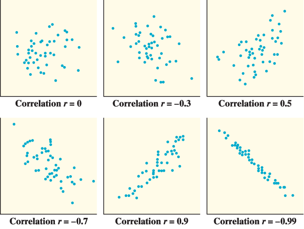
Strength (correlation): #
- A scatterplot can show a weak, moderate, or strong association.
- An association is strong if the points don’t deviate much from the form identified.
- An association is weak if the points deviate quite a bit from the form identified.
- Correlation doesn’t imply causation.
- In many cases, two variables might have a strong correlation, but changes in one variable are very unlikely to cause changes in the other variable
- ‘r’ — Correlation Coefficie
- It is only appropriate to use the correlation to describe strength and direction for a linear relationship
- Has same sign (positive or negative) as the slope
- r measures the direction and strength of the association, and does not measure form
- The correlation r is always a number between −1 and 1 (−1 ≤ r ≤ 1)
- The correlation r indicates the direction of a linear relationship by its sign: r > 0 for a positive association and r < 0 for a negative association.
- The extreme values r = −1 and r = 1 occur only in the case of a perfect linear relationship, when the points lie exactly along a straight line.
- If the linear relationship is strong, the correlation r will be close to 1 or −1. If the linear relationship is weak, the correlation r will be close to 0.
Unusual features: #
- outliers
- that fall outside the overall pattern and distinct clusters of points — doesn’t follow trend
- large residual
- definition link
- influential point
- if you remove the point, then there would be substantial changes on slope, y-int, or r
Interpreting #
There is a [strength — fairly strong/weak], [direction — positive / negative] [form — (non)linear] relationship between [x var] and [y-var] with [any outliers + outlier point].
Residuals #
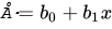
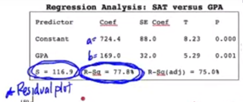 a = y-int, b = slope, s = s, R-sq = .$r^2$
Least-squares Regression Line (LSRL) #
- A regression line is a line that describes how a response variable y changes as an explanatory variable x changes.
- Made to reduce the residual
- Regression lines are expressed in the form where ŷ(pronounced “y-hat”) is the predicted value of y for a given value of x.
- Extrapolation is the use of a regression line for prediction far outside the interval of x values used to obtain the line. Such predictions are often not accurate.
- Don’t make predictions using values of x that are much larger or much smaller than those that actually appear in your data.
- Interpretation — NEEDS CONTEXT
- y-int
y=b0+b1*x
- b0
For a [context of x-var] with a [x-unit] of 0, the predicted [y-var] is [b0]
- Slope

- b1
For every increase of 1 in [x-unit], the predicted [y-unit] increases by [b1] [y-units]
- y-int
y=b0+b1*x
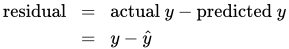
- Residual

- Difference between actual and predicted value
- Interpretation:
The actual [y-var] for a [context] of [x-input & x-units] is [actual value (point we know) - predicted value] [lower/higher] than predicted by the LSRL.
- Plug in respective values to LSRL to get the predicted value
- Residual Plot
- a scatterplot that displays the residuals on the vertical axis and the explanatory variable on the horizontal axis.
- To determine whether the regression model is appropriate, look at the residual plot.
- If there is no leftover curved pattern in the residual plot, the regression model is appropriate.
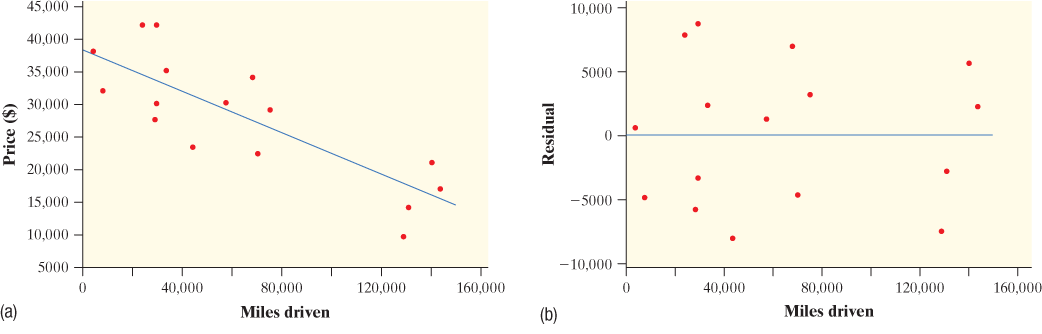 LSRL is good
 - Interpretation:
Because the residual plot does not show a clear pattern, the linear model is appropriate for the data
- If there is a leftover curved pattern in the residual plot, consider using a regression model with a different form.
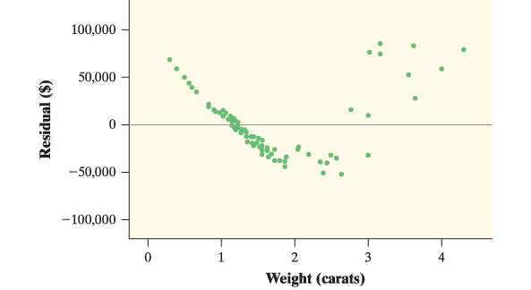 LSRL is bad
 - Interpretation:
Because the residual plot shows a clear patter, the linear model is not appropriate for the data
- If there is no leftover curved pattern in the residual plot, the regression model is appropriate.
Standard deviation of residuals: .$s$ #
- The standard deviation of the residuals s measures the size of a typical residual.
- That is, s measures the typical distance between the actual y values and the predicted y values.
- Interpretation:
The actual [y-var] [units] is typically around [s] away from the predicted by the least-squares regression line with x = [x-units]
The coefficient of determination: .$r^2$ #
- The coefficient of determination .$r^2$ measures the percent reduction in the sum of squared residuals when using the least-squares regression line to make predictions, rather than the mean value of y.
- In other words, .$r^2$ measures the percent of the variability in the response variable that is accounted for by the least-squares regression line.
- Interpretation:
About [.$r^2$ in percent form]% of the variability for [y-var] is accounted for by the least-squares regression line with x = [x-var]
Unit 3: Collecting Data #
Chapter 4
Sampling #
- The population in a statistical study is the entire group of individuals we want information about.
- A census collects data from every individual in the population.
- A sample is a subset of individuals in the population from which we collect data.
- A sample survey is a study that collects data from a sample that is chosen to represent a specific population.
Poor Sampling #
- Convenience sampling selects individuals from the population who are easy to reach.
- Voluntary response sampling allows people to choose to be in the sample by responding to a general invitation
- Bias:
- any difference between the sample result and the truth about the population that tends to occur in the same direction whenever you use the same sampling method
- The design of a statistical study shows bias if it is very likely to underestimate or very likely to overestimate the value you want to know.
- Bias is not just bad luck in one sample, it’s the result of a bad study design that will consistently miss the truth about the population in the same way
- If you’re asked to describe how the design of a sample survey leads to bias, you’re expected to do two things:
- Describe how the members of the sample might respond differently from the rest of the population
- Explain how this difference would lead to an underestimate or overestimate.
- Suppose you were asked to explain how using your statistics class as a sample to estimate the proportion of all high school students who own a graphing calculator could result in bias. You might respond, “This is a convenience sample . It would probably include a much higher proportion of students with a graphing calculator than in the population at large because a graphing calculator is required for the statistics class. So this method would probably lead to an overestimate of the actual population proportion.”
- Undercoverage
- occurs when some members of the population are less likely to be chosen or cannot be chosen in a sample.
- Most samples suffer from some degree of undercoverage. A sample survey of households, for example, will miss not only homeless people but also prison inmates and students in dormitories.
- Nonresponse
- Nonresponse occurs when an individual chosen for the sample can’t be contacted or refuses to participate
- Nonresponse leads to bias when the individuals who can’t be contacted or refuse to participate would respond differently from those who do participate.
- Consider a telephone survey that asks people how many hours of television they watch per day. People who are selected but are out of the house won’t be able to respond.
- Response Bias
- Response bias occurs when there is a systematic pattern of inaccurate answers to a survey question.
- The way questions are worded or the order in which they’re asked can lead to response bias
Good Sampling #
- Simple random sample (SRS)
- Involves using a chance process to determine which members of a population are included in the sample .
- Gives each possible sample an equal chance of being selected
- A simple random sample (SRS) of size n is chosen in such a way that every group of n individuals in the population has an equal chance to be selected as the sample.
- For example, to choose a random sample of 6 students from a class of 30, start by writing each of the 30 names on a separate slip of paper, making sure the slips are all the same size. Then put the slips in a hat, mix them well, and pull out slips one at a time until you have identified 6 different students.
- Strata, Stratified random sample
- Strata are groups of individuals in a population who share characteristics thought to be associated with the variables being measured in a study.
- good for when sample sizes between population groups (stratas) are different
- Stratified random sampling selects a sample by choosing an SRS from each stratum and combining the SRSs into one overall sample.
- For example, in a study of sleep habits on school nights, the population of students in a large high school might be divided into freshman, sophomore, junior, and senior strata. After all, it is reasonable to think that freshmen have different sleep habits than seniors. The following activity illustrates the benefit of choosing appropriate strata.
- Clusters, Cluster sampling
- A cluster is a group of individuals in the population that are physically located near each other.
- Cluster sampling selects a sample by randomly choosing clusters and including each member of the selected clusters in the sample .
- Cluster sampling is often used for practical reasons, like saving time and money.
- Imagine a large high school that assigns students to homerooms alphabetically by last name, in groups of 25. Administrators want to survey 200 randomly selected students about a proposed schedule change. It would be difficult to track down an SRS of 200 students, so the administration opts for a cluster sample of homerooms. The principal (who knows some statistics) selects an SRS of 8 homerooms and gives the survey to all 25 students in each homeroom.
- Systematic Random Sampling
- In systematic random sampling, the researcher first randomly picks the first item or subject from the population . Then, the researcher will select each n’th subject from the list.
- The procedure involved in systematic random sampling is very easy and can be done manually. The results are representative of the population unless certain characteristics of the population are repeated for every n’th individual, which is highly unlikely.
Experiments #
- Goal is to reduce bias and allow replication with the hopes that we find statistically significant results that we can infer/extrapolate to the population
- Four conditions of Experimental Design
- Comparison. Use a design that compares two or more treatments.
- Random assignment. Use chance to assign experimental units to treatments. Doing so helps create roughly equivalent groups of experimental units by balancing the effects of other variables among the treatment groups.
- Control. Keep other variables the same for all groups, especially variables that are likely to affect the response variable. Control helps avoid confounding and reduces variability in the response variable.
- Replication. (more than one experimental unit in each treatment group) — Use enough experimental units in each group so that any differences in the effects of the treatments can be distinguished from chance differences between the groups.
- Study:
- Observational Study: observes individuals and measures variables of interest but does not attempt to influence the responses.
- Observational Study vs experiment
- experiment (randomly) assigns treatments
- in studies the researcher has no interaction/input whatsoever
- data is observed and recorded naturally, scientists had no say
- can reduce bias from scientists
- no random assignment of subjects, but random sample can be taken
- therefore, we can make inferences about the population from which the individuals were chose, but not about cause and effect ( link)
- Vocab
- Experiment: deliberately imposes some treatment on individuals to measure their responses
- Response / Explanatory / Confounding Variables
- Placebo: A placebo is a treatment that has no active ingredient, but is otherwise like other treatments.
- The placebo effect describes the fact that some subjects in an experiment will respond favorably to any treatment, even an inactive treatment.
- Control: In an experiment, control means keeping other variables constant for all experimental units.
- Treatment: A specific condition applied to the individuals in an experiment
- Control group
- In an experiment, a control group is used to provide a baseline for comparing the effects of other treatments.
- Depending on the purpose of the experiment, a control group may be given an inactive treatment (placebo), an active treatment, or no treatment at all.
- Experimental unit: the object to which a treatment is randomly assigned
- Subjects: When the experimental units are human beings, they are often called subjects.
- Factor: In an experiment, a factor is a variable that is manipulated and may cause a change in the response variable.
- Levels: In an experiment, a factor is a variable that is manipulated and may cause a change in the response variable. The different values of a factor are called levels.
- Blinds
- In a double-blind experiment, neither the subjects nor those who interact with them and measure the response variable know which treatment a subject received.
- In a single-blind experiment, either the subjects don’t know which treatment they are receiving or the people who interact with them and measure the response variable don’t know which subjects are receiving which treatment
- Replication
- In an experiment, replication means using enough experimental units to distinguish a difference in the effects of the treatments from chance variation due to the random assignment.
- Sampling Variability
- Refers to the fact that different random samples of the same size from the same population produce different estimates.
- Larger random samples tend to produce estimates that are closer to the true population value than smaller random samples. In other words, estimates from larger samples are more precise.
- Statistically significant
- When the observed results of a study are too unusual to be explained by chance alone, the results are called statistically significant.
- Types of Experiments
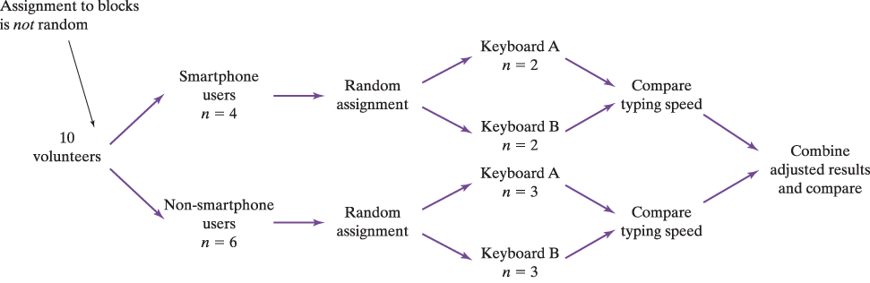
- Block, Randomized block design
- A block is a group of experimental units that are known before the experiment to be similar in some way that is expected to affect the response to the treatments.
- In a randomized block design, the random assignment of experimental units to treatments is carried out separately within each block.
- Matched Pairs
- A matched pairs design is a common experimental design for comparing two treatments that uses blocks of size 2.
- In some matched pairs designs, two very similar experimental units are paired and the two treatments are randomly assigned within each pair.
- In others, each experimental unit receives both treatments in a random order.
- Random Assignment: In an experiment, random assignment means that the treatment / placebo is randomly given out
- Block, Randomized block design
- Scope of Inference
- Inference: The process of drawing conclusions about a population based on samples, since we infer information about the population from what we know about the samples.
- Random Selection — sample units are selected randomly
- allows inference about the population from which the individuals were chosen
- groups may not be representative of population
- includes studies
- Random Assignment — experimental units are assigned to treatments using a chance process.
- allows inference about cause and effect.
- groups may differ between studies if not randomly assigned
- tend to average out all other uncontrollable factors so that they aren’t confounding with the treatment effects
- not studies
- Additional Requirements:
- The association is strong.
- The association is consistent.
- Larger values of the explanatory variable are associated w/ stronger responses.
- The alleged cause precedes the effect in time.
- Criteria for Establishing Causation When an Experiment CANNOT Be Done ● The association is strong. ● The association is consistent. ● Larger values of the explanatory variable are associated w/ stronger responses. ● The alleged cause precedes the effect in time. ● The alleged cause is plausible.
- Ethics
- All planned studies must be reviewed in advance by an institutional review board charged with protecting the safety and well-being of the subjects.
- All individuals who are subjects in a study must give their informed consent before data are collected.
- All individual data must be kept confidential. Only statistical summaries for groups of subjects may be made public.
Unit 4: Probability, Random Variables, and Probability Distributions #
Chapters 5 & 6
Probability #
- LAW OF LARGE NUMBERS
- A law that states if we observe more and more repetitions of any chance process, the proportion of times a specific outcome occurs approaches its actual probability.
- We cannot accurately predict outcomes in the SHORT RUN; Order only emerges in the LONG RUN.
- No such thing as Law of Averages – Only Law of Large Numbers!!!!!
- Probibility
- The probability of any outcome of a chance process is a number between 0 and 1 that describes the proportion of times the outcome would occur in A VERY LONG SERIES OF REPETITIONS.
- Outcomes that will never ever occur Probability = 0
- Outcomes that will always occur Probability = 1
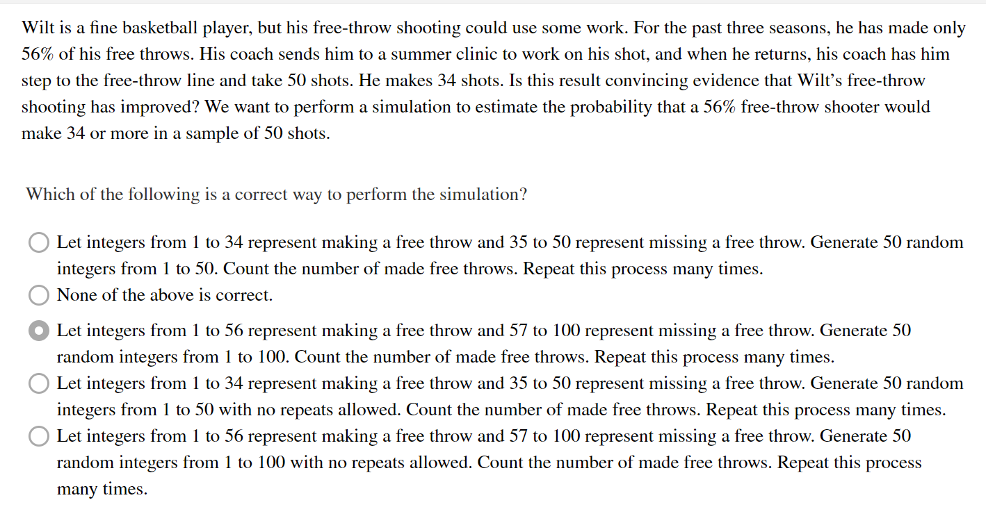
- Simulation
- The imitation of chance behavior, based on a model that accurately reflects the situation.
- The Simulation Process
- Describe how to use a chance device to imitate one trial (repetition) of the simulation.
Tell what you will record at the end of each trial.
- Remember that every label needs to be the same length. In the golden ticket lottery example, the labels should be 01 to 95 (all two digits), not 1 to 95.
- When sampling without replacement, be sure to mention that repeated numbers should be ignored.
- Perform many trials of the simulation.
- Use the results of your simulation to answer the question of interest.
- Example
- Describe how to use a chance device to imitate one trial (repetition) of the simulation.
Tell what you will record at the end of each trial.
- Probability Model: A description of some chance process that consists of 2 parts:
- a list of all possible outcomes
- SAMPLE SPACE: The list of all possible outcomes.
- the probability for each outcome
- a list of all possible outcomes
- EVENT Any collection of outcomes from some chance process — A subset of the entire sample space.
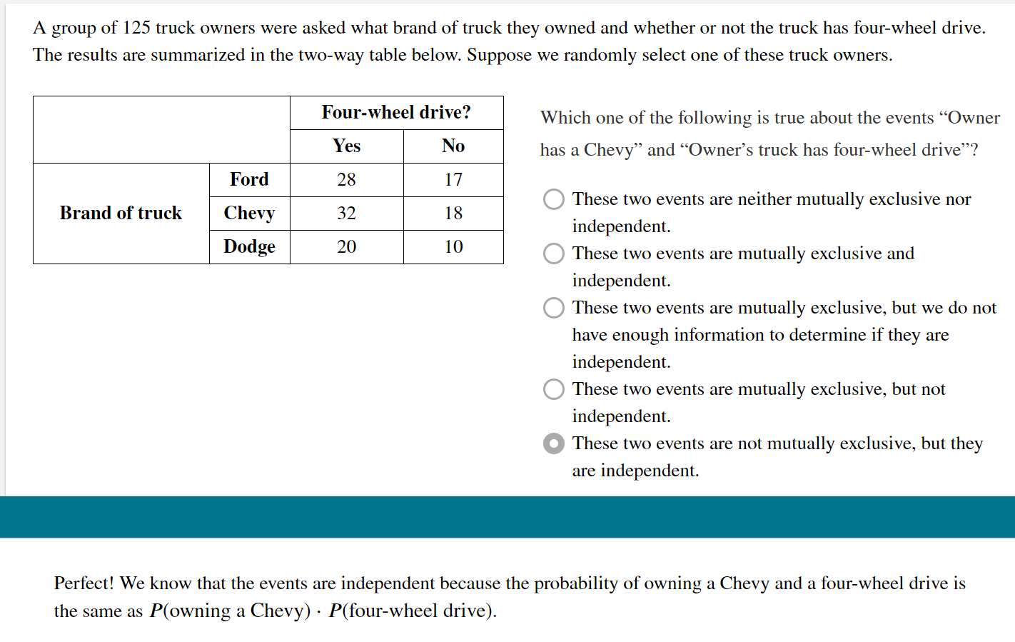
- MUTUALLY EXCLUSIVE Two events A & B are mutually exclusive if they have no outcomes in common and so can never occur together – that is, if P(A and B) = 0.
- General Rules $$0 ≤ P(A) ≤ 1 \text{ for any event }A$$ $$P(S) = 1 \text{ if }S\text{ is the sample space in a probability model}$$ $$P(A)=\frac{\text{Number of outcomes in event } A}{\text{Total number of outcomes in sample space}}\text{ in the case of EQUALLY LIKELY outcomes,}$$ $$\text{Complement Rule: } P(A^c)=1-P(A); \text{where }A^c=\text{the event that A does not occur}$$ $$\text{Addition rule for mutually exclusive events: }P(A \text{ or } B)=P(A \cup B) = P(A) + P(B)$$ $$\text{General addition rule: } P(A \text{ or } B) =P(A \cup B)= P(A) + P(B) − P(A \text{ and } B) $$ $$\text{Dependent events: } P(A \text{ and } B) = P(A ∩ B) = P(A) ⋅ P(B | A)$$ $$\text{Independent events: } P(A \text{ and } B) = P(A ∩ B) = P(A) ⋅ P(B)$$ $$\text{Probability of A given B: } P(A|B)=\frac{P(A \text{ and } B)}{P(B)} $$
- Conditional
- CONDITIONAL PROBABILITY
- Example
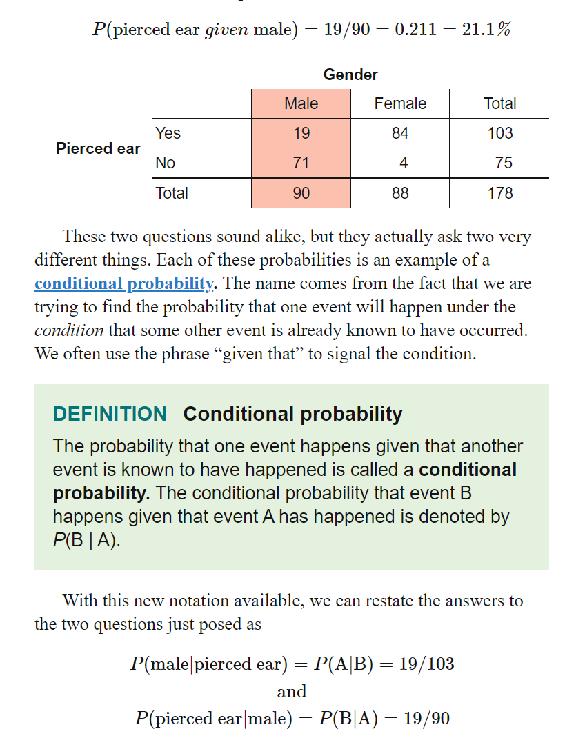
- The probability that one event happens given that another event is known to have happened.
- The conditional probability that event B happens GIVEN that event A has happened is denoted by P(B | A).
- Example
- CONDITIONAL PROBABILITY
- INDEPENDENT EVENTS
- A and B are independent events if knowing whether or not one event has occurred does not change the probability that the other event will happen.
- In other words, events A and B are independent if $$P(A ∣ B) = P(A ∣ B ^c ) = P(A)$$
- Alternatively, events A and B are independent if $$P(B ∣ A) = P(B ∣ A^c) = P(B)$$
- A and B are independent events if knowing whether or not one event has occurred does not change the probability that the other event will happen.
Random Variables #
- DISCRETE RANDOM VARIABLE
- A random variable that has a countable number of outcomes with gaps.
- Examples: ACT Scores; # of Free-Throws Made, etc.
- CONTINUOUS RANDOM VARIABLE
- A random variable that has an infinite number of outcomes with no gaps.
- Examples: Temperature; Race Times; Heart Rate, etc.
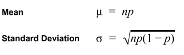
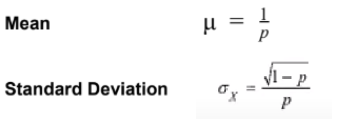
- Mean

- Variance

- Standard Deviation
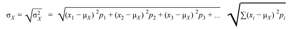
- Transforming — only works for independent!
- When MULTIPLYING (or DIVIDING) each value in a probability distribution by some number b, the ● mean is MULTIPLIED (or DIVIDED) by b ● variance is MULTIPLIED (or DIVIDED) by b^2 ● standard deviation is MULTIPLIED (or DIVIDED) by b
- When ADDING (or SUBTRACTING) the number a to each value in a probability distribution, the ● mean INCREASES (or DECREASES) by a ● variance STAYS THE SAME ● standard deviation STAYS THE SAME
- Combining — only works for independent!
Suppose we add two normal distributions (X + Y) or we subtract two normal distributions (X – Y). The shape of the resulting distribution will be NORMAL and the mean and standard deviation can be calculated using the RULES.
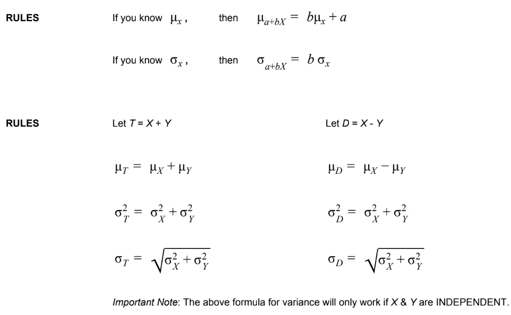 where \row (no ^2) is standard deviation
 - Difference between the binomial setting and the geometric setting

- Binomial
- Binomial Setting:
- Binary? Each observation falls into 1 of 2 categories: SUCCESS or FAILURE
- Independent? The n observations are all INDEPENDENT. (knowing one outcome of a trial has no effect on the other trials)
- Note: if sampling w/o replacement, you need to check the 10% condition
- Number? There is a fixed number n of TRIALS/OBSERVATIONS.
- Success? The probability of success, p, is SAME for each trial.
- BINOMIAL DISTRIBUTION
- If large counts is verified, then the binomial distribution’s shape is approximately normal
- The distribution of the count X of successes in the binomial setting with parameters n and p.
- n = # of Trials/Observations
- p = Probability of Success (per Trial)
- Possible Values for X = whole #s 0 to n
- Abbreviation = B (n, p)
- BINOMIAL COEFFICIENT
- The number of ways to arrange k successes among n trials; “Combinations”
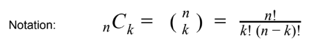
- The number of ways to arrange k successes among n trials; “Combinations”
- Binomial Probability Formula
binomialPdf/Cdfalso works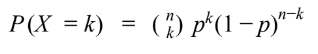
- Binomial Setting:
- Geometric:
- The Geometric Setting
- Binary? Each observation falls into 1 of 2 categories: SUCCESS or FAILURE
- Independent? The n observations are all INDEPENDENT. (knowing one outcome of a trial has no effect on the other trials).
- Trials? The goal is to count the number of trials until the FIRST SUCCESS
- Success? The probability of success, p, is SAME for each trial.
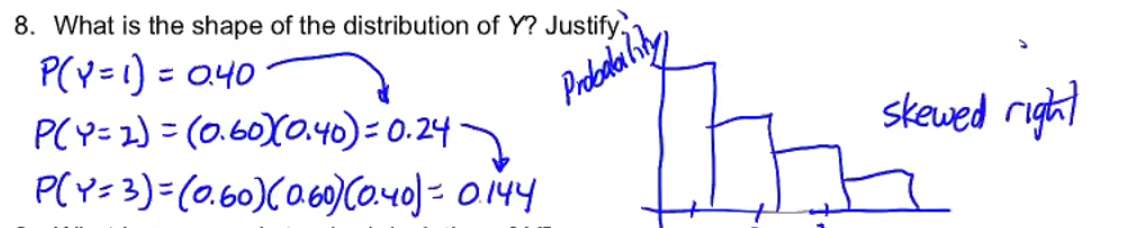
- Shape
- skewed right
- skewed right
- GEOMETRIC PROBABILITY FORMULA
geometCdf/Pdfalso works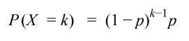
- The Geometric Setting
Unit 5: Sampling Distributions #
Chapter 7 + 10
Sampling Distribution: #
- The sampling distribution of a statistic is the distribution of values taken by the statistic in all possible samples of the same size from the same population.
- Always say “the distribution of [blank],” being careful to distinguish the distribution of the population, the distribution of sample data, and the sampling distribution of a statistic.
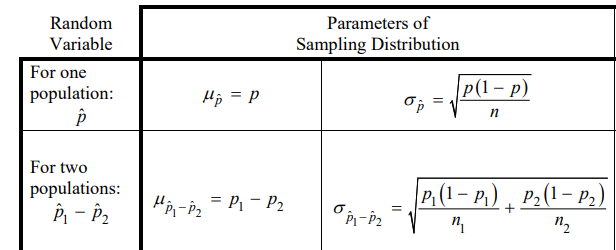
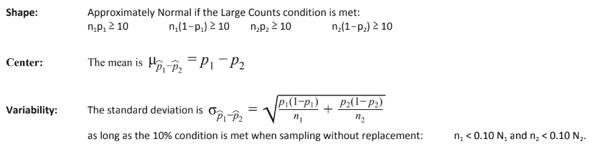
- Sampling distribution of the sample proportion
- The sampling distribution of the sample proportion p hat describes the distribution of values taken by the sample proportion p hat in all possible samples of the same size from the same population.
- Conditions
- Random: The data must come from a well-designed RANDOM sample or a RANDOMIZED experiment.
- Normal: The sampling distribution is approximately NORMAL, meaning we can use a z-test statistic.
- Large Counts: (np ≥ 10) & (n (1 − p) ≥ 10 )
- Independent:
- If 2 samples, both samples must be independent
- 10% Condition: When sampling w/o replacement to verify the use of our standard deviation ( 10n < N )
- The sampling distribution of the sample proportion p hat describes the distribution of values taken by the sample proportion p hat in all possible samples of the same size from the same population.
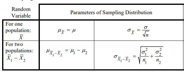
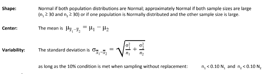
- Sampling distribution of the sample mean
- The sampling distribution of the sample mean x describes the distribution of values taken by the sample mean x in all possible samples of the same size from the same population.
- Conditions
- Random: The data must come from a well-designed RANDOM sample or a RANDOMIZED experiment.
- Normal: The sampling distribution is approximately NORMAL, meaning we can use a z-test/t-test statistic.
- Either (or both) condition(s) must be met:
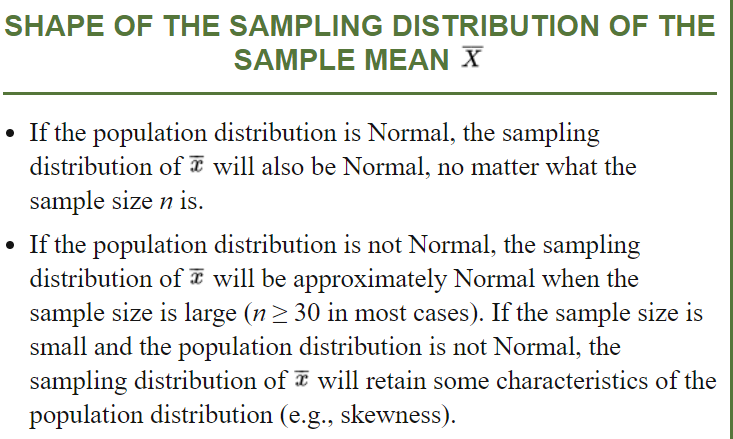
- CLT
- n ≥ 30 — n_diff ≥ 30 for paired data
- The central limit theorem (CLT) says that when n is larger than 30, the sampling distribution of the sample mean x is approximately Normal.
- Distribution shouldn’t be skewed
- values above the median are much more variable than the values below the median
- values above the median are much more variable than the values below the median
- Independent:
- If 2 samples, both samples must be independent
- 10% Condition: When sampling w/o replacement to verify the use of our standard deviation ( 10n < N ) — 10*n_diff < N_diff for paired data
- The sampling distribution of the sample mean x describes the distribution of values taken by the sample mean x in all possible samples of the same size from the same population.
- Sampling Variability: Sampling variability refers to the fact that different random samples of the same size from the same population produce different values for a statistic.
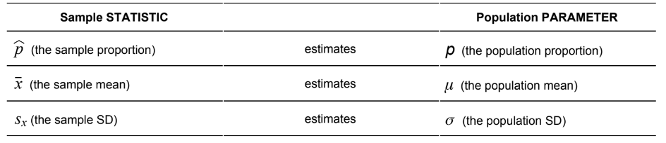
- Parameter: A number computed from a population
- Statistic
- A number computed from a SAMPLE
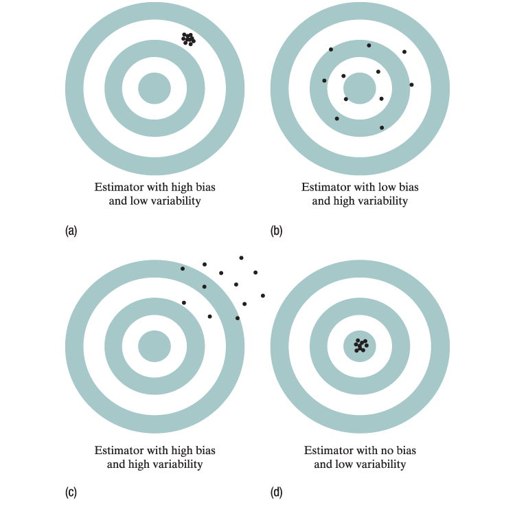
- What makes a statistic a good estimator of a parameter?
- LOW BIAS (Randomization) High bias is usually because of a poor sampling design (lack of randomness).
- LOW VARIABILITY (Sample Size) Reduce the variability of a statistic is to INCREASING SAMPLE SIZE.
- Difference between proportions
- Difference between means
 Many students use “accurate” when they really mean “precise.” For example, a response that says “increasing the sample size will make an estimate more accurate” is incorrect
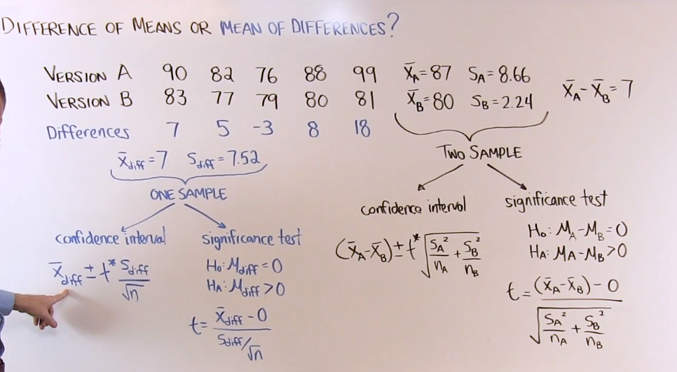
Paired Data #
- Paired data result from recording two values of the same Quantitative variable for each individual or for each pair of similar individuals.
- 2 sets of data that are not independent from each other, then they’re paired
- Analyzing Paired Data:
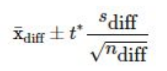
- To analyze paired data, start by computing the difference for each pair. Then make a graph of the differences. Use the mean difference x and the standard deviation of the differences as summary statistic.
Confidence Intervals #
- Point estimator:
- a statistic that provides an estimate of a population parameter.
- The value of that statistic from a sample is called a point estimate.
- Ideally our “best guess” at the value of an unknown parameter.
- Because the sample mean ¯x is an unbiased estimator of the population mean μ, we use the statistic ¯x as a point estimator ****of the parameter μ. The best guess for the value of μ is ¯x
- Unbiased Estimator: A statistic used to estimate a parameter is an unbiased estimator if the mean of its sampling distribution is equal to the value of the parameter being estimated.
- Confidence Level α
- The confidence level C% gives the overall success rate of the method used to calculate the confidence interval.
- Interpretation
If we were to select many random samples from a population and construct a C% confidence interval using each sample, about C% of the intervals would capture the [parameter in context].
- Confidence interval

- When interpreting a confidence interval, make sure that you are describing the parameter and not the statistic.
- Interpretation
“We are C% confident that the interval from [min] to [max] captures the true value of the [parameter in context].”
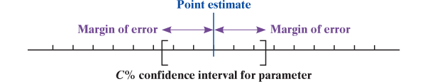
- Margin of error
- describes how far, at most, we expect the estimate to vary from the true population value.
- In a C% confidence interval, the distance between the point estimate and the true parameter value will be less than the margin of error in C% of all samples.
- How to decrease MOE
- The confidence level decreases. To obtain a smaller margin of error from the same data, you must be willing to accept less confidence.
- The sample size n increases. In general, increasing the sample size n reduces the margin of error for any fixed confidence level.
- Margin of error accounts for only the variability we expect from random sampling. It does not account for practical difficulties, such as undercoverage and nonresponse in a sample survey
- Critical Value
- The critical value is a multiplier that makes the interval wide enough to have the stated capture rate.
- Z-score when we know stdiv
- t-score when we don’t know stdiv
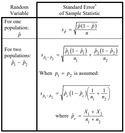
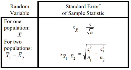
- Standard Error (SE)
Proportions #
- Four-step process:
- State
- What parameter do you want to estimate and at what confidence level?
- 1 proportion
“We wish to estimate the true proportion of all [parameter], with [C%] confidence.”
- 2 proportions
“We wish to estimate the true difference of the proportion of all [parameter 1] and all [parameter 2] for [context], with [C%] confidence.”
- Plan
- Identify the appropriate inference method
“We’ll carry out a [ONE/TWO]-SAMPLE Z INTERVAL FOR A POPULATION PROPORTION (because we’re estimating a proportion and we know the standard deviation.)”
- Check conditions
- Identify the appropriate inference method
- Do
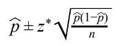
- Perform the calculations.
“Because the conditions are true, we can do our calculations:”
- 1 proportion
- 2 proportions
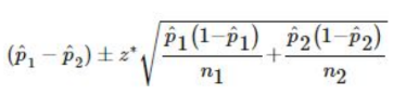
- where z* is the critical value for the standard Normal curve with C% of its area between −z* and z*.
- Conclude
- Interpret your interval in the context of the problem.
We are [C%] confident that the interval of [min] to [max] [units] captures the true proportion of all [context]
- 2 sample difference
- If 0 is within confidence interval range:
Because 0 is contained in the [C%] confidence interval it is plausible there is no difference between [parameter 1] and [parameter 2]. We do not have convincing evidence of a difference of proportions of [context]
- If 0 is NOT within confidence interval range:
Because 0 is not contained in the [C%] confidence interval it is plausible there is a difference between [parameter 1] and [parameter 2]. We have convincing evidence of a difference of proportions of [context]
- If 0 is within confidence interval range:
- Interpret your interval in the context of the problem.
- State
Means #
- Four-step process
- State
- What parameter do you want to estimate and at what confidence level?
- 1 proportion
We wish to estimate the true mean of all [parameter], with [C%] confidence.
- 2 proportions
We wish to estimate the true difference of the mean of all [parameter 1] and all [parameter 2] for [context], with [C%] confidence.
- Plan
- Identify the appropriate inference method
- If we know stdiv
We’ll carry out a [ONE/TWO]-SAMPLE Z INTERVAL FOR A POPULATION MEAN(because we know the standard deviation.)
- If we don’t know stdiv
We’ll carry out a [ONE/TWO]-SAMPLE Z INTERVAL FOR A POPULATION MEAN(because and we don’t know the standard deviation.)
- If we know stdiv
- Check conditions
- Identify the appropriate inference method
- Do
- Perform the calculations.
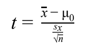
- z-score
Because we know conditions are true, can do our calculations
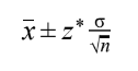
- 1 mean
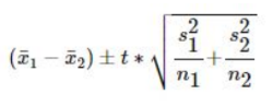
- 2 means
 with z* score and \row
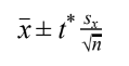
- 1 mean
- t-score
Because we know conditions are true, we can say that the t-distribution’s degree of freedom (df) is df = n - 1 and we’ll carry out a [one/two]-sample t interval for a population mean
- 1 mean
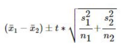
- 2 means
- Difference
- 1 mean
- Conclude
- Interpret your interval in the context of the problem.
We are [C%] confident that the interval of [min] to [max] [units] captures the true mean of all [context]
- 2 sample difference
- If 0 is within confidence interval range:
Because 0 is contained in the [C%] confidence interval it is plausible there is no difference between [parameter 1] and [parameter 2]. We do not have convincing evidence of a difference between means of [context]
- If 0 is NOT within confidence interval range:
Because 0 is not contained in the [C%] confidence interval it is plausible there is a difference between [parameter 1] and [parameter 2]. We have convincing evidence of a difference between means of [context]
- If 0 is within confidence interval range:
- Interpret your interval in the context of the problem.
- State
- t-scores
- A t-distribution is specified by its degrees of freedom (df) calculated df = n - 1
- The spread of the t-distribution is MORE than that of a standard Normal distribution.
- The t-distribution has MORE probability in the tails than the standard Normal distribution, since substituting the estimate sx for the parameter σ introduces MORE variation into the statistic.
- As degrees of freedom increases, the t-distribution becomes CLOSER to the standard Normal distribution, since sx estimates MORE accurately when the sample size is large.
Choosing sample size #
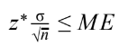
- Sometimes, we want to choose our sample size (n) so that we may estimate a proportion within a particular margin of error. We must choose our sample size before we start sampling.
- Conservative Approach: Use p .5 , because it maximizes the margin of error.
- Better Approach if Possible: Make a guess about the value of p based on prior knowledge, common knowledge, previous studies, etc. $$Z^*\sqrt{\frac{p(1-p)}{n}} \leq ME, \text{and solve for n}$$
- Sample Size for a Desired Margin of Error when Estimating μ
- To determine the sample size n that will yield a C% confidence interval for a population mean with a specified margin of error ME:
- Get a reasonable value for the population standard deviation σ from an earlier or pilot study.
- Find the critical value z* from a standard Normal curve for confidence level C%.
- Set the expression for the margin of error to be less than or equal to ME and solve for n:
- To determine the sample size n that will yield a C% confidence interval for a population mean with a specified margin of error ME:
Tests #
Shared Vocab #
- Significance Test
- A formal procedure for comparing OBSERVED DATA with a CLAIM whose truth we want to assess.
- Null hypothesis — H0
- A test is designed to assess the strength of the evidence AGAINST this.
- This hypothesis is often the statement of “no difference.”
- Alternative hypothesis — Ha
- The claim about the population we are trying to find evidence FOR.
- This hypothesis should always be created BEFORE seeing the data.
- One sided
- less than or greater than
- Two sided
- not equal
- Both Null & Alternative Hypotheses refer to a POPULATION and use PARAMETERS (μ & p)
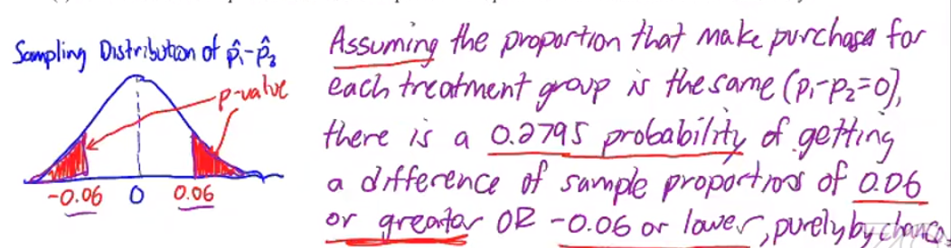
- p-value
- Assuming H0 is true, the probability the statistic (such as p^hat or x^bar) would take a value as extreme or more extreme than the one actually observed.
- The smaller the p-value, the STRONGER the evidence is AGAINST the H0
- Interpretation
“Assuming H0 is true, there is a [P-val] probability of getting the [sample val] [or even smaller/larger] by random chance with a sample size of [n]”
- significance level
- The level at which that, when our p-value falls below it, we consider it to be SIGNIFICANT
- We consider that our sample is so unlikely to happen IF H0 is true, that it likely did NOT happen by chance
- error + power
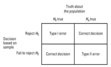
- Type 1:
- When H0 is true, but we REJECT H0
- P(Type I) = confidence level α
- Type 2:
- When Ha is true, but we FAIL TO REJECT H0
- P(Type II) = 1 - Power
- Power
- The ability of a test to correctly detect the alternative when it’s true.
- When Ha is true, and we CORRECTLY REJECT H0
- Interpretation
“Given Ha is true (in context), there is a (power) probability we correctly rejecting H0 (finding convincing evidence for Ha)
- Power = 1 – P(Type II Error)
- How to increase
- INCREASE the sample size (n),
- INCREASE the Confidence Level (α), or
- Make Ha further away from H0
- The ability of a test to correctly detect the alternative when it’s true.
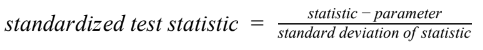
- STANDARDIZED TEST STATISTIC
- A standardized test statistic measures how far a sample statistic is from what we would expect if the null hypothesis H0 were true, in standard deviation units.
- A standardized test statistic measures how far a sample statistic is from what we would expect if the null hypothesis H0 were true, in standard deviation units.
- Type 1:
Proportions #
- Four-step process
- State
- State your Hypotheses: H[relation] = [p/µ]
- interpret values — 1 proportion
where p is the true proportion of [context] and Significance Level (alpha)
- interpret values — 2 proportion
where p is the true difference between the proportions of [parameter 1] and [parameter 2] of [context] and Significance Level (alpha)
- Plan
- Identify the appropriate testing method
We’ll carry out a [ONE/TWO]-SAMPLE Z TEST FOR A POPULATION PROPORTION (because we’re estimating a proportion and we know the standard deviation)
- Check conditions
- Identify the appropriate testing method
- Do
- Perform the calculations.
Because we know conditions are true, can do our calculations
- 1 sample
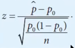
- 2 sample
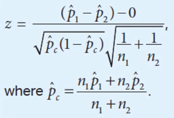 Proportion Difference
 - find p-value
- Perform the calculations.
- Conclude
- Interpret your p-value in the context of the problem.
- P-value less than
Assuming the [H0] is true, there is a [p-value] probability of getting [statistic found] or [more [and/neither] less — more for H0 < Ha; less for Ha < H0; both for H0 ≠ Ha] in a sample of [sample size] purely by chance. Because [p-value] is less than [alpha] of [confidence level], we have evidence to reject the null hypothesis, and have some evidence that the null hypothesis may be true, meaning [context]
- P-value greater than
Assuming the [H0] is true, there is a [p-value] probability of getting [statistic found] or [more [and/neither] less — more for H0 < Ha; less for Ha < H0; both for H0 ≠ Ha] in a sample of [sample size] purely by chance. Because [p-value] is greater than [alpha] of [confidence level], we do not have enough evidence to reject the null hypothesis, meaning [context]
- P-value less than
- Interpret your p-value in the context of the problem.
- State
Means #
- Four-step process
- State
- State your Hypotheses: H[relation] = [p/µ]
- interpret values — 1 proportion
where p is the true mean of [context] and Significance Level (α)
- interpret values — 2 proportion
where p is the true difference between the means of [parameter 1] and [parameter 2] of [context] and Significance Level (α)
- Plan
- Identify the appropriate testing method
We’ll carry out a [[ONE/TWO]-SAMPLE]/MATCHED PAIRS] T TEST FOR A POPULATION MEAN
- Check conditions
- Identify the appropriate testing method
- Do
- Perform the calculations.
Because we know conditions are true, can do our calculations with (n-1) degrees of freedom
- 1 sample
- 2 sample
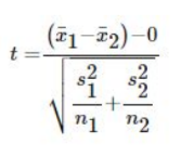 Mean Difference
 - Paired
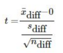 Paired
 - find P-value
- Perform the calculations.
- Conclude
- Interpret your p-value in the context of the problem.
- P-value less than
Assuming the parameter is true, there is a [p-value] probability of getting [statistic found] or more/less in a sample of [sample size] purely by chance. Because [p-value] is less than [alpha] of [confidence level], we have evidence to reject the null hypothesis, and have some evidence that the null hypothesis may be true, meaning [context]
- P-value greater than
Assuming the parameter is true, there is a [p-value] probability of getting [statistic found] or more/less in a sample of [sample size] purely by chance. Because [p-value] is greater than [alpha] of [confidence level], we do not have enough evidence to reject the null hypothesis, meaning [context]
- P-value less than
- Interpret your p-value in the context of the problem.
- State