01-25: Gaussian Elimination, Vectors #
Upper Triangular Systems #
- Consider the following equation $$x-y+2z=1$$ $$y-z=2$$ $$z=1$$
…which can be represent as an augmented matrix: $$\begin{bmatrix} 1 & -1 & 2 & \text{|} & 1\\ 0 & 1 & -1 & \text{|} & 2\\ 0 & 0 & 1 & \text{|} & 1 \end{bmatrix}$$
- These are called
upper triangle matrices – they are nice in that they’re easy to solve!
- The solution is reached when the diagonal is all one, the remaining is zero (excluding the rightmost ‘answer’ colum)
Row Echelon Form #
- More precisely, a matrix is in
row echelon form when the following criteria are met:
- All nonzero rows are above all zero rows.
- The leading coefficient of a non-zero row is always to the right of the leading coefficient of the row above it.
$$\begin{bmatrix} 1 & * & * & * & \text{|} & *\\ 0 & 1 & * & * & \text{|} & *\\ 0 & 0 & 0 & 1 & \text{|} & *\\ 0 & 0 & 0 & 0 & \text{|} & 0 \end{bmatrix}$$
- The leading coefficient of every non-zero row (which we call the pivot, and say is in the pivot position) is 1.
- Some textbooks will require this third property, others don’t
Reduced Row Echelon Form #
- Reduced Row Echelon Form: requires that, in addition to the upwards propagation of variables in step (3), we will obtain a matrix with the following properties, in addition to the two mentioned above:
- The matrix is in row echelon form.
- The leading coefficient of every non-zero row (which we call the pivot, and say is in the pivot position) is 1.
- Each column with an element that is in the pivot position of some row has 0s everywhere else.
$$\begin{bmatrix} 1 & 0 & * & 0 & \text{|} & *\\ 0 & 1 & * & 0 & \text{|} & *\\ 0 & 0 & 0 & 1 & \text{|} & *\\ 0 & 0 & 0 & 0 & \text{|} & 0\\ \end{bmatrix}$$
- Sometimes abbreviated (especially in programming) as
rref. - By construction, the Gaussian elimination algorithm always results in a matrix that is in reduced row echelon form.
- Once an augmented matrix is reduced to reduced row echelon form, variables corresponding to columns containing leading entries are called basic variables, and the remaining variables are called free variables
- If there just isn’t enough information and the equations do not contradict each other, then there exist an infinite number of solutions.
- When this happens, choose some variable (ideally, which is in most of the equations) and then solve each equation in terms of that variable (e.x. .$z$ is in all equations, so now write .$x,y,\dots$ in terms of .$z$).
- Once an augmented matrix is reduced to reduced row echelon form, variables corresponding to columns containing leading entries are called basic variables, and the remaining variables are called free variables
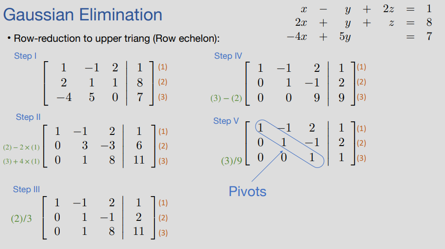
Example
We start with the following system: $$x-y+2z=1$$ $$2x+y+z=8$$ $$-4x+5y = 7$$
…which we can write as a matrix $$\begin{bmatrix} 1 & -1 & 2 & \text{|} & 1\\ 2 & 1 & 1 & \text{|} & 8\\ -4 & 5 & 0 & \text{|} & 7 \end{bmatrix}$$
…and we can row-reduce to upper triangle (Row echelon)
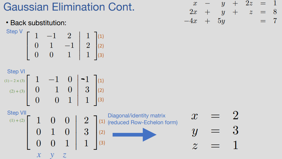
…which we can use back substitution to solve
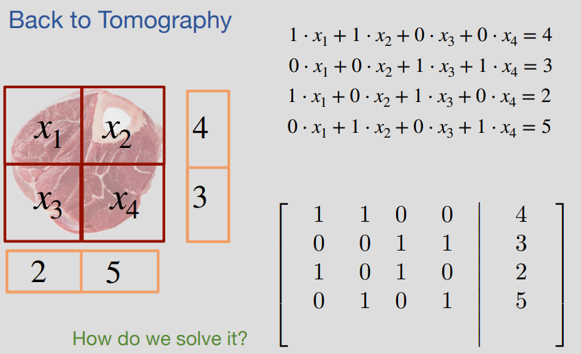
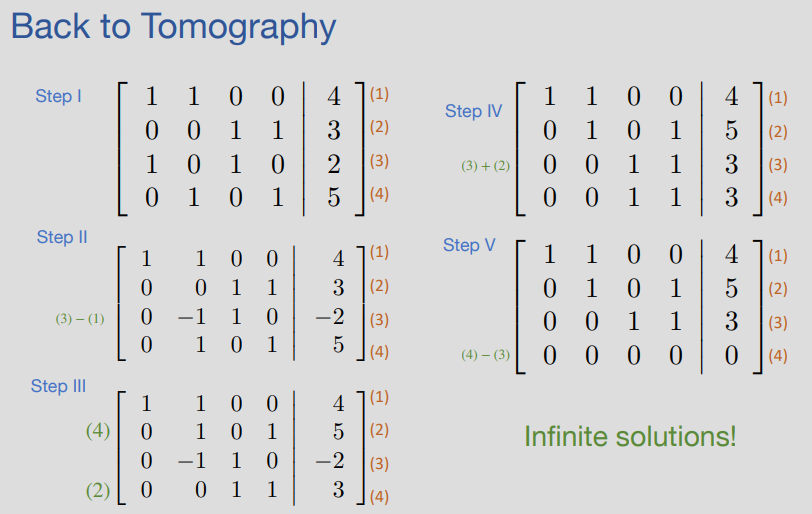
Tomograph Example

Error #
- In real systems, we will always have noise (error) that makes our systems slightly skewed
- So what if we repeat the example above, but have a measurement of .$+0.1$… are there any solutions?
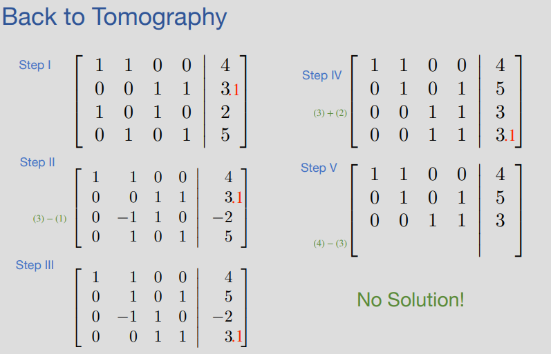
- So what if we repeat the example above, but have a measurement of .$+0.1$… are there any solutions?
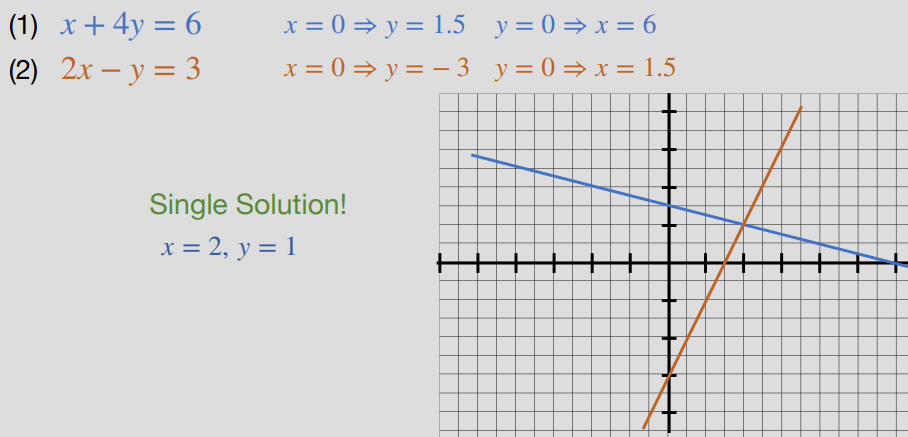
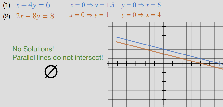
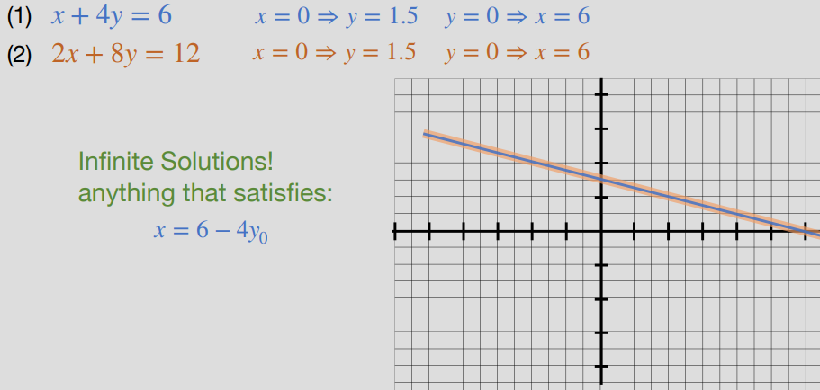
Graphing #
- We can represent our solution as a set of linear equations, meaning we can represent them graphically
01-27: Vectors, Matrices, Multiplications, And Span #
Last lecture, we showed how vectors and matrices could be used as a way of writing systems of linear equations more compactly, demonstrating through our tomography example that modeling a set of measurements as a system of equations can be a powerful tool.
In these following notes, we are going to more thoroughly discuss how to perform computations with vectors and matrices. In future notes, we will consider additional properties of vectors and matrices and see how these can help us understand real-world systems.
Vectors #
- Given a collection of .$n$ real numbers such as .$x_1, x_2, \dots x_n$, we can represent this collection as a single point in an .$n$-dimensional real space .$\mathbb{R}^n$, denoted as a .$\vec x$
- Each .$x_i$ (for .$i$ between .$1$ and .$n$) is called a component, or element, of the vector.
$$\vec x = \begin{bmatrix} x_1 \\ x_2 \\ \vdots \\ x_n \end{bmatrix}$$
- The size of a vector is the number of components it contains
- Two vectors .$\vec x$ and .$\vec y$ are said to be equal, .$\vec x = \vec y$, if they have the same size and .$x_i = y_i$ for all .$i$
- Vectors are interesting because they can represent any set of numbers
- Representing as vectors lets us apply a lot of nice operations to them + represent them graphically
- In Tomography, we can write a vector to represent the amount of light absorbed by each bottle in a row or column.
- E.x. color (RGB values), pictures (set of pixels), solar cycles, Electrical circuit quantities
Vectors Representing State #
- Vectors can be used to represent the state of a system, defined as follows:
State: The minimum information you need to completely characterize a system at a given point in time, without any need for more information about the past of the system.
- State is a powerful concept because it lets us separate the past from the future.
- The state completely captures the present– and the past can only affect the future through the present
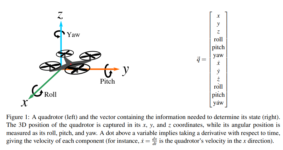
- E.x: Consider modeling the dynamics of a quadrotor. The state of a quadrotor at a particular time can be summarized by its 3D position, angular position, velocity, and angular velocity, which can be represented as a vector .$\vec q \in \mathbb{R^{12}}$, as illustrated:
Special vectors #
Zero & One Vector: #
- You can usually tell the size of the zero from the context: if .$\vec x \in \mathbb{R}^{n}$ is added to .$\vec 0$, then .$\vec 0$ must also be in .$\mathbb{R}^{n}$
$$\vec 0 = \begin{bmatrix} 0 \\ 0 \\ \vdots \\ 0 \end{bmatrix}$$
$$\vec 1 = \begin{bmatrix} 1 \\ 1 \\ \vdots \\ 1 \end{bmatrix}$$
Standard Unit Vector: #
- A standard unit vector is a vector with all components equal to .$0$ except for one element, which is equal to .$1$. A standard unit vector where the .$i$th position is equal to .$1$ is written as .$\vec e_i$
- The system .$e_1, \dots, e_n \in \mathbb{R}^{n}$ is called the standard basis in .$\mathbb{R}^{n}$
$$\vec e_1 = \begin{bmatrix} 1 \\ 0 \\ \vdots \\ 0 \end{bmatrix},\ \vec e_2 = \begin{bmatrix} 0 \\ 1 \\ \vdots \\ 0 \end{bmatrix},\ \vec e_n = \begin{bmatrix} 0 \\ 0 \\ \vdots \\ 1 \end{bmatrix}$$
- When talking about standard unit vectors in the context of states, we might also use the word “pure” to refer to such states. This is because they only have one kind of component in them. Other states are mixtures of pure states.
Vector Operations #
Addition #
- Must be same size and space (e.g. complex numbers, real numbers, etc.)
- Properties:
- Many of the properties of addition you are already familiar with when adding individual numbers hold for vector addition as well. For three vectors .$\vec x, \vec y, \vec z \in \mathbb{R}^n$ (and .$\vec 0 \in \mathbb{R}^n$), the following properties hold:
- Commutativity: $$\vec x + \vec y = \vec y + \vec x$$
- Additive identity: $$\vec x + 0 = \vec x$$
- Associativity: $$(\vec x + \vec y) + \vec z = \vec x + (\vec y + \vec z)$$
- Additive inverse: $$\vec x + (- \vec x) = 0$$
- Many of the properties of addition you are already familiar with when adding individual numbers hold for vector addition as well. For three vectors .$\vec x, \vec y, \vec z \in \mathbb{R}^n$ (and .$\vec 0 \in \mathbb{R}^n$), the following properties hold:
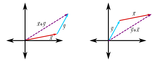
- Vector addition can be performed graphically as well:
Scalar Multiplication #
- We can multiply a vector by a number, called a scalar:
Scalar: a number. In mathematics and physics, scalars can be used to describe magnitude or used to scale things (e.g. cut every element of a vector in half by multiplying by 0.5, or flip the signs of each element in a vector by multiplying by −1).
- In general, for a scalar .$\alpha$ and vector .$\vec x$, this looks like this: $$\alpha \begin{bmatrix} x_1 \\ x_2 \\ \vdots \\ x_n \end{bmatrix} = \begin{bmatrix} \alpha x_1 \\ \alpha x_2 \\ \vdots \\ \alpha x_n \end{bmatrix} $$
- We can obtain the zero vector by multiplying any vector by 0: $$0\vec x = \vec 0$$
- Properties:
- Associative, distributive, and multiplicative identity hold – trivial
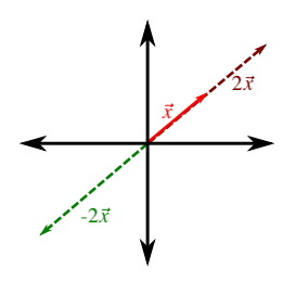
- As an example, we can scale a vector .$\vec x \in \mathbb{R}^{2}$ by 2 or -2:
Vector Transpose #
- .$\vec x$ is always a column vector, so to convert (represent) a row vector, we apply the transpose: .$\vec x^T$
- If the elements of the matrix .$A \in \mathbb{R}^{N \times M}$ are .$a_{ij}$
- The elements of .$A^T \in \mathbb{R}^{M \times N}$ are .$a_{ji}$
- Matrix transpose is not (generally) an inverse!
$$\vec x = \begin{bmatrix} x_1 \\ x_2 \\ \vdots \\ x_N \end{bmatrix}; \vec x \in \mathbb{R}^{N \times 1}$$ $$\vec x^T = \begin{bmatrix} x_1 & x_2 & \dots & x_N \end{bmatrix}; \vec x^T \in \mathbb{R}^{1 \times N} $$
- The transpose of a row vector is a column vector
- Thus, the transpose of the transpose of a vector recovers the original vector.
- It is important to recognize that, though the transpose of a vector contains the same elements as the original vector, it is still a different vector!
- That is to say, for any vector .$\vec x$ (with at least two components), .$\vec x ^T \neq \vec x$
- The transpose of a matrix has a very nice interpretation in terms of linear transformations, namely it gives the so-called adjoint transformation.
Vector-Vector Multiplication #
- By convention, a row vector can only be multiplied by a column vector (and vice versa).
- Multiplication is valid only for specific matching dimensions!
- Width of the first, matches length of the second’s transpose
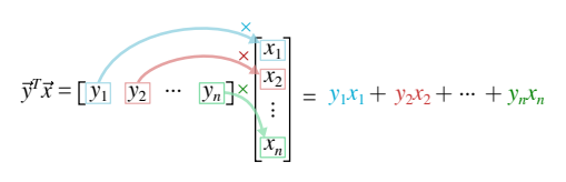
- e.x. given .$\vec x, \vec y \in \mathbb{R}^{N\times 1}$
- We can take the transpose of .$y$ and multiply by .$\vec x$:
- This is also known as inner product or dot product
- Commutative for real numbers (this ceases to be true when we start working with complex numbers in 16B)
$$\vec y^T \vec x = y_1 x_1 + y_2 x_2 + \dots + y_N x_N = \text{some scalar} \in \mathbb{R}^{1\times1}$$
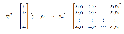
- Alternatively, we can take .$\vec x$ and multiply by the transpose of .$y$
- Also known as outer product
- Do not commute!
$$\vec x \vec y^T = \text{some matrix} \in \mathbb{R}^{N \times N}$$
- We can take the transpose of .$y$ and multiply by .$\vec x$:
Matrices #
- A collection of numbers in a rectangular form
- Or, given .$\mathbb{R}^{M \times N}$, a collection of .$M$ rows and .$N$ column vectors
- Remark: Matrices are often represented by capital letters (e.g. .$A$),
$$A = \begin{bmatrix} a_{11} & \dots & a_{1N} \\ \vdots & \ddots & \vdots\\ a_{M1} & \dots & a_{MN} \end{bmatrix}$$
- A matrix is said to be square if .$M=N$ (that is, if the number of rows and number of columns are equal).
- Relation between scalars, vectors, and matrices
- A vector is a degenerate matrix, that is, .$\vec x \in \mathbb{R}^{n \times 1}$
- A scalar is a degenerate vector or matrix, that is, .$a \in \mathbb{R}^{1 \times 1} $
- Transpose:
- Just as we could compute the transpose of a vector by transforming rows into columns, we can compute the transpose of a matrix, .$A^T$ , where the rows of .$A^T$ are the (transposed) columns of .$A$
$$A^T = \begin{bmatrix} a_{11} & \dots & a_{M1} \\ \vdots & \ddots & \vdots\\ a_{1N} & \dots & a_{NM} \end{bmatrix}$$
- Mathematically, .$A^T$ is the .$N\times M$ matrix given by .$A^T_{ij}$
- A square matrix is said to be symmetric if .$A = A^T$ , which means that .$A_{ij} = A_{ji}$ for all .$i, j$.
Special Matrices #
- Zero Matrix: Trivial
- Identity Matrix: Square matrix whose diagonal elements are .$1$ and whose off-diagonal elements are all .$0$
$$I_3 = \begin{bmatrix} 1 & 0 & 0 \\ 0 & 1 & 0\\ 0 & 0 & 1 \end{bmatrix}$$
- Note that the column vectors (and the transpose of the row vectors) of an .$N \times N$ identity matrix are the unit vectors in .$ \mathbb{R}^{N}$. The identity matrix is useful because multiplying it with a vector .$\vec x$ will leave the vector unchanged: .$I \vec x = \vec x$.
- In fact, we will see that multiplying a square matrix by an identity matrix of the same size will yield the same initial matrix: .$AI = IA = A$
Column vs Row #
The interpretation of rows and columns that come from the system-of-linear-equations perspective of doing experiments. There, each row of the matrix represents a particular experiment that took one particular measurement. For a given row, the coefficient entries represent how much the corresponding state variable affects the outcome of this particular experiment. In contrast, the columns represent the influence of a particular state variable on the collection of experiments taken together. These perspectives come in handy in interpreting matrix multiplication.
Matrix Operations #
Matrix Addition #
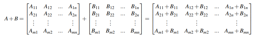
- Two matrices of the same size can be added together by adding their corresponding components. For instance, we can add two matrices A and B (both in .$ \mathbb{R}^{m \times n}$) as follows:
Matrix-Vector Multiplication #
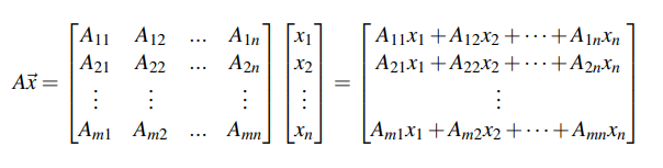
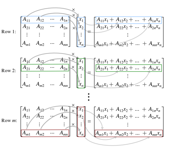
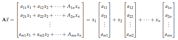
- Given .$A \in \mathbb{R}^{M \times N}, \vec x = \mathbb{R}^{N\times 1}$, we end with some vector .$\in \mathbb{R}^{M\times 1}$
Visual View
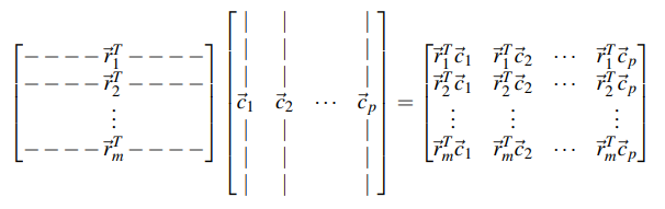
Matrix-Matrix Multiplication #
- Matrix-Matrix multiplication involves multiplying each row vector in .$A$ with each column vector in .$B$, starting from the top row of matrix .$A$ and leftmost column of matrix .$B$.
- Effectively, the left matrix is multiplied by each column vector in the second matrix to produce a new column of .$AB$
- Given .$A \in \mathbb{R}^{M \times N},\ B = \mathbb{R}^{N\times L}$, we end with some matrix .$\in \mathbb{R}^{M \times L}$
- We can also interpret the .$A \vec x$ product in the context of .$A$’s columns:
- Matrix multiplication does not commute!
- That is .$A \times B \neq B \times A$
- In fact, both quantities can only be calculated if the number of rows in .$A$ equals the number of columns in .$B$ and the number of rows in .$B$ equals the number of columns in .$A$.
- Matrix Multiplication is Associative
- Fun fact: Computers have to do so many multiply and add operations that it’s optimized at a processor level (leaned about this is 61C)