23.1 Electric Potential Energy and Difference #
- PE can only be defined for conservative forces
- That is, work done by said force is independent of the path taken
- Coulomb’s Law is conservative because the dependence on position is conservative
- Hence, we define .$\Delta U = -W$ with
- .$\Delta U = U_b - U_a$ is for a situation where a point charge .$q$ moves from point .$a$ to point .$b$
- This is equal to negative work, .$-W = -\vec F d = -(q\vec E) d$ (for a uniform .$\vec E$)
23.2 Relation between Electric Potential and Field #
- Electric Potential: Electric PE per unit charge, such as for a charge at point .$a$ $$V_a = \frac{U_a}{q}$$
- We only really care about difference though, which is defined as $$V_{ba} = \Delta V = \frac{U_b - U_a}{q} = - \frac{W_{ba}}{q}$$
- We can now also define PE in terms of electric potential: $$\Delta U = U_b - U_a = q(V_b - V_a) = qV_{ba}$$
- Electric potential difference is a measure of how much energy an electric charge can acquire in a given situation.
- Since energy is the ability to do work, the electric potential difference is also a measure of how much work a given charge can do.
- The exact amount of energy or work depends both on the potential difference and on the charge.
- If a positive charge is free, it will tend to move from high to low potential
- Inverse for opposite charge
23.3 Potential due to Point Charges #
$$\Delta U = U_b - U_a = - \int_a^b \vec F \cdot d \vec l$$
- .$dl$ is an infinitesimal increment of displacement along the path from .$a$ to .$b$
- Keep in mind that .$\vec F$ must be conservative
- Thus the integral can be taken along any path from point .$a$ to point .$b$.
- Knowing .$\vec E = \vec F / q$ and .$V_{ba} = (U_b - U_a) / q$, we can write the electric potential equation as…
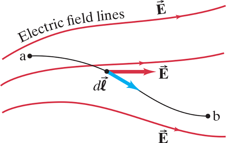
$$V_{ba} = V_b - V_a = - \int_a^b \vec E \cdot d \vec l$$ $$V_{ba, \text{uniform $\vec E$}} = -E\int_a^b d\vec l = -Ed$$ …where .$d$ is the distance of a straight line from point .$a$ to .$b$
Charged Conducting Sphere #
1. Electric Potential Outside Sphere #
- We know .$\vec E = \frac{1}{4\pi\varepsilon_0} \frac{Q}{r^2}$ for outside a conducting sphere (.$r > r_0$)
- Therefore, we can write $$V_{ba} = - \int_{r_a}^{r_b} \vec E \cdot d \vec l = - \frac{Q}{4\pi\varepsilon_0}\int_{r_a}^{r_b} \frac{dr}{r^2}$$ $$\dots = \frac{Q}{4\pi\varepsilon_0} \bigg(\frac{1}{r_b} - \frac{1}{r_a}\bigg)$$ $$\dots = \frac{1}{4\pi\varepsilon_0} \frac{Q}{r} \text{ [$r_b = \infty$]}$$
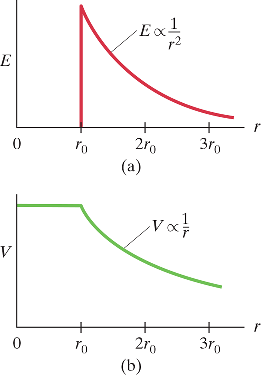
2. Electric Potential On Sphere #
- From .$(a)$, as .$r$ approaches .$r_0$, we see $$V = \frac{1}{4\pi\varepsilon_0} \frac{Q}{r_0}$$ at the surface of the sphere. This makes sense because the charge is distributed on the surface of the sphere.
3. Electric Potential Inside Sphere #
- Inside the conductor, .$\vec E = 0$
- Therefore, there is no change in .$\vec E$ from .$0$ to .$r_0$ (or any point within the conductor) gives zero change in .$V$
- Hence, within the conductor, .$V$ is a constant: $$V = \frac{1}{4\pi\varepsilon_0} \frac{Q}{r_0}$$
- Thus, the whole conductor, not just its surface, is at this same potential.
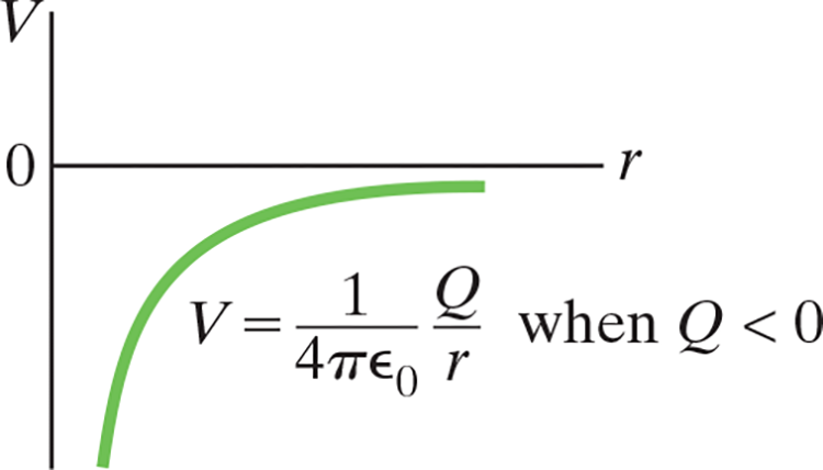
- We can also generalize the first case to the electric potential .$r$ from a single point charge .$Q$
Coulomb potential #
- The potential outside a uniformly charged sphere is the same as if all the charge were concentrated at its center
The potential near a positive charge is large, and it decreases toward zero at very large distances

For a negative charge, the potential is negative and increases toward zero at large distances
23.4 Potential due to Any Charge Distribution #
- If .$\vec E$ is a function of position (or otherwise unknown), we can find .$V$ by calculating the potential due to the many tiny charges that make up .$\vec E$: $$V = \frac{1}{4\pi\varepsilon_0} \int \frac{dq}{r}$$ where .$r$ is the distance from a tiny element of charge .$dq$ to the point where .$V$ is being determined
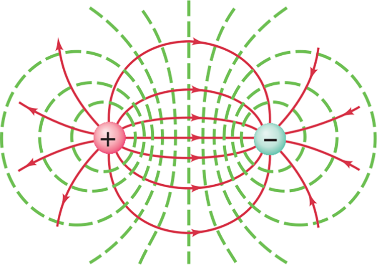
23.5 Equipotential Lines and Surfaces #
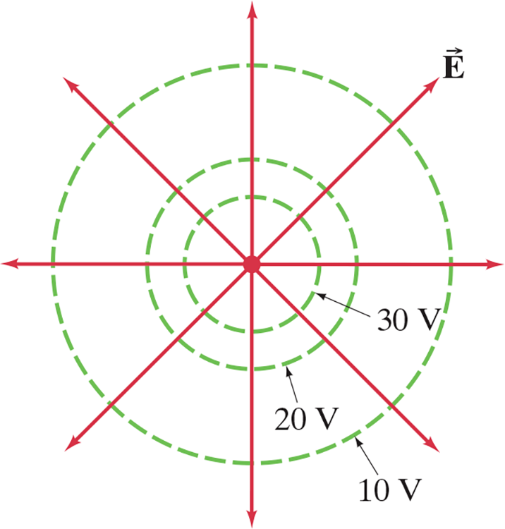
- The electric potential can be represented by drawing equipotential lines, or, in three dimensions, equipotential surfaces
- An equipotential surface has all points at the same potential.
- That is, the potential difference between any two points on the surface is zero
- Thus, no work is required to move a charge from one point on the surface to another.
- Equipotential surfaces are perpendicular to the electric field (field lines)
- For a positive point charge, the equipotential surface with the largest potential is closest to the positive charge
- Unlike electric field lines, which start and end on electric charges, equipotential lines/surfaces are always continuous and never end
Electric field lines and equipotential surfaces for a point charge.
Equipotential lines (green, dashed) are always perpendicular to the electric field lines (solid red) shown here for two equal but oppositely charged particles (an electric dipole).
23.6 Potential Due to Dipole (Moment) #
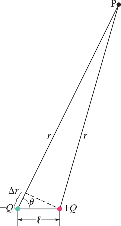
$$V = \frac{1}{4\pi\varepsilon_0} \frac{Q}{r} + \frac{1}{4\pi\varepsilon_0} \frac{(-Q)}{(r+\Delta r)} = \frac{Q}{4\pi\varepsilon_0} \frac{\Delta r}{r(r + \Delta r)}$$
- .$r$ is the distance from (some arbitrary point) .$P$ to the positive charge and .$r + \Delta r$ is the distance to the negative charge
- If .$r \gg l$, then .$r \gg \Delta r \approx l \cos \theta$ so we can neglect .$\Delta r$ $$V = \frac{1}{4\pi\varepsilon_0} \frac{Ql \cos\theta}{r^2} = \frac{1}{4\pi\varepsilon_0} \frac{p \cos\theta}{r^2} $$
- Notice the potential decreases .$\propto r^2$, whereas for a single point charge the potential decreases .$\propto r$
- It is not surprising that the potential should fall off faster for a dipole:
- When you are far from a dipole, the two equal but opposite charges appear so close together as to tend to neutralize each other
23.7 .$\vec E$ Determined from .$V$ #
- We know that .$V_b - V_a = - \int_a^b \vec E \cdot d\vec l$, which we can write in differential form as .$dV = -\vec E \cdot d\vec l = - E_l dl$. This can be written as $$E_l = - \frac{dV}{dl}$$
- .$dV$ is the tiny difference in potential between two points a distance .$dl$ apart, and .$E_l$ is the component of the electric field in the direction of the tiny displacement .$d\vec l$
- This is called the gradient of .$V$ in a particular direction: The general case is $$\vec E = - \nabla \vec V = - \bigg\langle \frac{\delta V}{\delta x}, \frac{\delta V}{\delta y}, \frac{\delta V}{\delta z} \bigg\rangle$$
- This states that the electric field points “downhill” towards lower voltages (where there is lower potential)
23.8 Electrostatic PE; The Electron Volt #
- The electric potential and energy potential due to one point charge .$Q_1$ on another point charge .$Q_2$ separated by .$r_{12}$ are $$V = \frac{1}{4\pi\varepsilon_0} \frac{Q_1}{r_{12}}$$ $$U = Q_2 V = \frac{1}{4\pi\varepsilon_0} \frac{Q_1 Q_2}{r_{12}}$$
- The PE is the negative work needed to separate the two charges to infinity.
- For three points, we can use the superposition principle like we have prior to write $$U = \frac{1}{4\pi\varepsilon_0}\bigg( \frac{Q_1 Q_2}{r_{12}}+ \frac{Q_1 Q_3}{r_{13}} + \frac{Q_2 Q_3}{r_{23}} \bigg)$$
Electron Volt #
- Joules are a very large unit for dealing with energy of the electron scale; as such, the electron volt (.$eV$) is often used
- One electron volt is the energy acquired by a particle carrying a charge .$e$ (the magnitude of an electron) as a result of moving through a potential difference of .$1 V$ $$1 \text{ eV} = 1.6022 \cdot 10^{-19} \text{ J}$$
- E.x., an electron (charge .$e = 1.6\cdot10^{-19}$) that accelerates through a potential difference of .$1000 \text{ V}$ will lose .$1000 \text{ eV}$ of potential energy and gain .$1000 \text{ eV}$ of kinetic energy
23.9 Digital; Binary Numbers; Signal Voltage (not covered) #
- Batteries and wall sockets provide a steady supply voltage as power
- Signal voltage provide/carry information
- Analog signal voltage has voltage that varies continuously (i.e .$\sin$)
- Digital signals are more complicated and encode information, often in binary
- Bytes have 8 bits which allow .$2^8 = 256$ numbers
- Digital signals are transmitted at some rate (bit-rate) given in .$\text{Mb/s}$
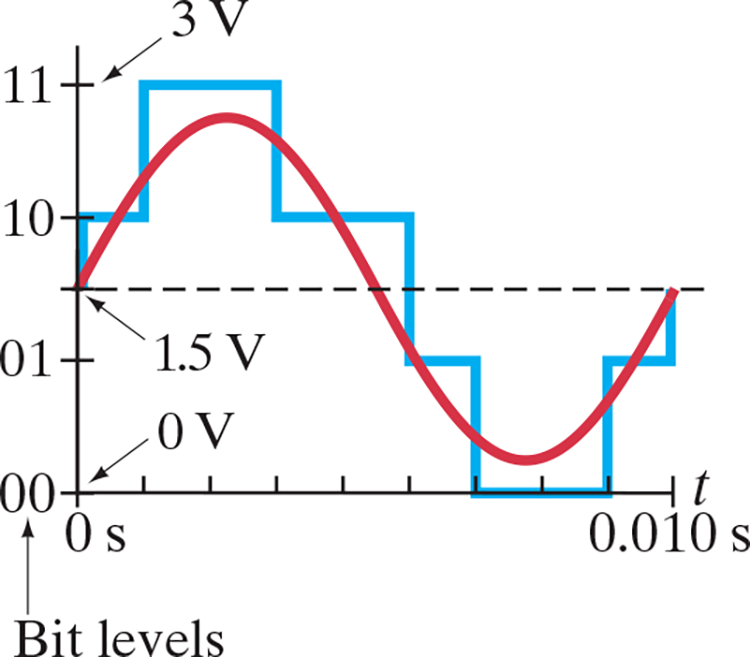
- Analog to digital converters, ADCs, convert analog signals to boxy digital waves
- The difference between the original continuous and it’s digital approximation is called the quantization error / loss
- This error varies by primarily:
- Resolution or bit depth which is the number of bits for the voltage of each sample
- Sampling rate which is the number of times per second the original analog voltage is measured (sampled)
- E.x., CDs are sampled at .$44.1 \text{ kHz}$ with a bit depth of .$16 \text{ bits per sample}$
The red analog sine wave, which is at a 100-Hz frequency (1 wavelength is done in 0.010 s), has been converted to a 2-bit (4 level) digital signal (blue).
- Digital Signals
- Digital to Analog, DACs, exist too because some appliances require an analog signal
- Digital signals can be compressed: Repeated information can be reduced so that less memory (bits) is needed
- Fun fact: Bit is the contraction of “binary digit”, leaving out the 8 letters between
- Digital signals are more resistant from noise, which badly corrupts analog signals
- Any electronic signal involves electric charges whose electric field can affect charges in another nearby signal
- External fields, as from high voltage wires, motors, or fluorescent lamps, can produce noise
- Thermal noise refers to random motion of electrons, much like the “thermal motion” of the molecules in a gas
- Moving electrons can be affected by the medium (wire, etc.), altering the signal