14.1 Functions of Several Variables #

• In the real world, most things don’t depend on a single variable
  • Temperature may depend on the .$(x,y)$ (latitude/longitude) position
  • Volume of a cylinder depends on radius .$r$ and height .$h$: .$V =\pi r^2 h$
• Formal Definition: A function .$f$ of two variables is a rule that assigns to each ordered pair of real numbers .$(x,y)$ in a set .$D$ a unique real number denoted by .$f(x,y)$. The set .$D$ is the domain of .$f$ and its range is the set of values that .$f$ takes on, that is, .$\{f(x,y)\ |\ (x,y) \in D \}$.
  • E.x. for .$f(x,y) = \frac{\sqrt{x+y+1}}{x-1}$, the domain is .$D = \{(x,y)\ |\ x + y + 1 \geq 0, x \neq 1\}$ which can be graphed with a solid line following .$y =-x-1$ with a dotted line at .$x = 1$
  • E.x. for .$f(x,y) = x\ln(y^2-x)$, the domain is .$D =\{(x,y)\ |\ x<y^2\}$. This can be graphed with a dotted line following the curve .$x = y^2$
• For the equation .$z = f(x,y)$, .$x,y$ are the independent variables and .$z$ is the dependent variable – similar to single variable equations
• We can visualize functions of two variables (i.e .$f(x,y)$) by graphing them in 3D as .$(x,y,f(x,y))$
  • We can then write level curves for the function by setting .$f(x,y) = k$ for some .$k$onstant in the range of .$f$. This will result in a graph similar to a Topographic map

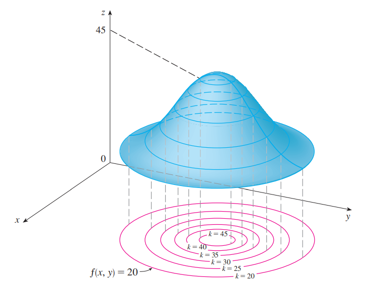
    Level Curve: The level curves of a function .$f$ of two variables are the curves with equations .$f(x,y) = k$, where .$k$ is a constant (in the range of .$f$).

14.2 Limits and Continuity #

Limits #

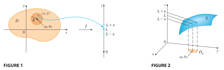
Vector Limit: Let .$f$ be a function of two variables whose domain .$D$ includes points arbitrarily close to .$(a, b)$. Then we say that the limit of .$f(x, y)$ as .$(x, y)$ approaches .$a, b.$ is .$L$ and we write $$\lim_{(x,y)\to(a,b)} f(x,y) = L$$ if for every number .$\varepsilon < 0$ there is a corresponding number .$\delta < 0$ such that if .$(x, y) \in D$ and .$0 < \sqrt{(x-a)^2 + (y-b)^2} < \delta$ then .$\vert f(x,y) - L \vert < \varepsilon$

• Notice that .$\vert f(x,y) - L \vert$ is the distance between the numbers .$f(x, y)$ and .$L$, and .$\sqrt{(x-a)^2 + (y-b)^2}$ is the distance between the point .$(x, y)$ and the point .$(a, b)$.
• If .$f(x,y) \to L_1$ as .$(x,y) \to (a,b)$ along a path .$C_1$ and .$f(x,y) \to L_2$ as .$(x,y) \to (a,b)$ along a path .$C_2$, where .$L_1 \neq L_2$, then .$\lim_{(x,y)\to(a,b)} f(x,y)$, does not exist.
  • We can test this by setting .$x$ and .$y$ to various different values (e.x. .$x = 0, y = 0, x = y, …,$ etc)

Continuity #

A function .$f$ of two variables is called continuous at .$(a,b)$ if $$\lim_{(x,y)\to (a,b)} f(x,y) = f(a,b)$$ We say .$f$ is continuous on .$D$ if .$f$ is continuous at every point .$(a,b)$ in .$D$.

• That is, we need the limit to exist ands for .$f(a,b)$ to be defined
• Continuous functions: .$x,y, c, \text{ trig (on domain)}$
• Arithmetic, composition, exponent all preserve continuity (on domain!)
• Dividing doesn’t necessarily preserve continuity

14.3 Partial Derivatives #

If .$f$ is a function of two variables, its partial derivatives are the functions .$f_x$ and .$f_y$ defined by $$f_x(x,y) = \frac{\delta f}{\delta x} = \lim_{h\to0} \frac{f(x+h,y)-f(x,y)}{h}$$ $$f_y(x,y) = \frac{\delta f}{\delta y} = \lim_{h\to0} \frac{f(x,y+h)-f(x,y)}{h}$$

• Notice we use .$\delta$ instead of .$d$ for partial derivatives
• These can be written at a single point .$(a,b)$ with respect to .$x$ and .$y$ by treating the remaining variables as a constant $$f_x(a,b) = g’(a); \ \ \ g(x) = f(x,b)$$ $$f_y(a,b) = h’(b); \ \ \ h(y) = f(a,y)$$
• Which can be extrapolated for 3 (or more) variables: $$f_z(a,b,c) = k’(c); \ \ \ k(z) = f(a,b,z)$$

Higher Derivatives #

• Just like regular derivatives, we can do many partial derivatives
• For example, the following are second partial derivatives of .$z = f(x,y)$: $$(f_x)_x = f_{xx} = \frac{\delta }{\delta x}\bigg(\frac{\delta f}{\delta x}\bigg) = \frac{\delta^2f}{\delta x^2}$$ $$(f_x)_y = f_{xy} = \frac{\delta }{\delta y}\bigg(\frac{\delta f}{\delta x}\bigg) = \frac{\delta^2f}{\delta y \delta x}$$ $$(f_y)_x = f_{yx} = \frac{\delta }{\delta x}\bigg(\frac{\delta f}{\delta y}\bigg) = \frac{\delta^2f}{\delta x \delta y}$$ $$(f_y)_y = f_{yy} = \frac{\delta }{\delta y}\bigg(\frac{\delta f}{\delta y}\bigg) = \frac{\delta^2f}{\delta y^2}$$

Clairaut’s Theorem Suppose .$f$ is defined on a disk .$D$ that contains the point .$(a,b)$. If the functions .$f_{xy}$ and .$f_{yx}$ are both continuous on .$D$, then $$f_{xy}(a,b) = f_{yx}(a,b)$$

Partial Differential Equations #

• In the sciences, we typically want to find how a system changes with respect to multiple variables
• Partial derivatives occur in partial differential equations, e.x Laplace’s Equation: $$ \frac{\delta^2 u}{\delta x^2} + \frac{\delta^2 u}{\delta y^2} = 0$$
  • Solutions to Laplace’s are always harmonic functions, such as .$u = e^x \sin(y)$

14.4 Tangent Planes and Linear Approximations #

Tangent Planes #

• Tangent planes are to surfaces as tangent lines are to curves
  • Tangent planes contain both the partial derivative lines w.r.t .$x$ and .$y$
• All we need to know to write a tangent plane is a point .$(a,b)$ and direction of the two partial derivatives .$\langle 1,0, f_x(a,b)\rangle, \langle 0,1, f_y(a,b)\rangle$
  • Direction vector can be found with .$\langle 1,0, f_x(a,b)\rangle \times \langle 0,1, f_y(a,b)\rangle = \langle -f_x, -f_y, 1 \rangle$ which we can dot with .$\langle x-x_0, y-y_0, z-f(x_0,y_0) \rangle$

    Suppose .$f$ has continuous partial derivatives. An equation of the tangent plane to the surface .$z = f(x, y)$ at the point .$P(x_0,y_0,z_0)$ is $$z-f(x_0, y_0) = f_x(x_0,y_0)(x-x_0) + f_y(x_0, y_0)(y-y_0)$$

Linear Approximations #

• As we get very close to the surface, then the tangent plane (at point .$(a,b)$) looks more and more like the surface
  • Thus, we can use it to for making approximations when we are near near .$(a,b)$

    If .$z = f(x,y)$, then .$f$ is differentiable at .$(a,b)$ if .$\Delta z$ can be expressed in the form $$\Delta z = f_x(a,b)\Delta x + f_y(a,b)\Delta y + \varepsilon_1 \Delta x + \varepsilon_2 \Delta y$$ where the error terms, .$\varepsilon_1$ and .$\varepsilon_2 \to 0$ as .$(\Delta x, \Delta y) \to (0,0)$ and the other terms are the linearization of the function.

• Rewriting this, we can use the given .$f(x,y)$ to write the linear approximation which is an estimate for point/state at .$f(a,b)$ $$f(x,y) \approx f(a,b) + f_x(a,b) (x-a) + f_y(a,b)(y-b)$$
• We can similarly define the 3D linear approximation, increment of .$w$, and differential .$dw$ as: $$f(x,y,z) \approx f(a,b,c) + f_x(a,b,c) (x-a) + f_y(a,b,c)(y-b) + f_z(a,b,c) (z-c)$$ $$\Delta w = f(x+\Delta x, y + \Delta y, z + \Delta z) - f(x,y,z)$$ $$dw = \frac{\delta w}{\delta x}dx + \frac{\delta w}{\delta y}dy + \frac{\delta w}{\delta z}dz$$

Differentials #

• With one variable functions, i.e. .$y = f(x)$, we defined the differential .$dx$ to be independent so we had to write .$dy$ as .$dy = f’(x)\ dx$
• Given a differentiable function of two variables, i.e. .$z = f(x,y)$, we know both .$dx$ and .$dy$ are independent so we write: $$dz = f_x(x,y)\ dx + f_y(x,y)\ dy = \frac{\delta z}{\delta x}dx + \frac{\delta z}{\delta y}dy$$
• If the partial derivatives .$f_x$ and .$f_y$ exist near .$(a,b)$ and are continuous at .$(a,b)$, then .$f$ is differentiable at .$(a,b)$.

14.5 Chain Rule #

Chain Rule #

Suppose that .$z = f(g_1 (x_1,_{\dots}, x_m), g_2 (x_1,_{\dots}, x_m), g_n (x_1,_{\dots}, x_m))$ is a differentiable function of the .$n$ variables .$g_1,_{\dots}, g_n$ and is .$g_j$ is a differentiable function of the .$m$ variables .$x_1,_{\dots}, x_m$. Then .$z$ is a function of .$x_1,_{\dots}, x_m$ and $$ \frac{\delta f}{\delta x_i} = \frac{\delta f}{\delta g_1} \frac{\delta g_1}{\delta x_i} + \frac{\delta f}{\delta g_2} \frac{\delta g_2}{\delta x_i} + \dots + \frac{\delta f}{\delta g_m} \frac{\delta g_m}{\delta x_i}$$ for each .$i = 1,2,\dots,m$

Implicit Differentiation #

• If .$F(x,y) = 0$ defines .$y$ implicitly as a function of .$x$ (that is, .$y = f(x)$, where .$F(x,f(x))= 0$ for all .$x$ in the domain of .$f$), then $$ \frac{dy}{dx} = - \frac{\frac{\delta F}{\delta x}}{ \frac{\delta F}{\delta y}} = - \frac{F_x}{F_y}$$

• If .$F(x,y,z) = 0$ defines .$z$ implicitly as a function of .$x,y$, then

$$ \frac{dz}{dx} = - \frac{\frac{\delta F}{\delta x}}{ \frac{\delta F}{\delta z}} = - \frac{F_x}{F_z};\ \ \frac{dz}{dy} = - \frac{\frac{\delta F}{\delta y}}{ \frac{\delta F}{\delta z}} = - \frac{F_y}{F_z}$$

14.6 Directional Derivatives and the Gradient Vector #

Directional Derivatives #

Direction Derivative For function .$f$ at .$(x_0, y_0)$ in the direction of unit vector .$\hat u = \langle a, b \rangle$ is $$D_{\hat u} f(x_0, y_0) = \lim_{h\to 0} \frac{f(x_0 + ha, y_0 + hb) - f(x_0, y_0)}{h} = $$ $$\dots = \nabla f \cdot \hat u = f_x (x,y) a + f_y (x,y) b$$ if the limit exists (for the former) and if .$f$ is a differentiable function of .$x$ and .$y$ (for the latter)

• That is, .$\hat u = \hat i = \langle 1, 0 \rangle$ for .$D_\hat{i} = f_x$ and .$\hat u = \hat j = \langle 0, 1 \rangle$ for .$D_\hat{j} = f_y$
• Differentiability is important because it means that as you approach the surface very closely, it looks more and more like the tangent plane.
• Directional derivatives can be thought of as the slope of the tangent line at a given point
• This definition can be extrapolated to (three variables/higher dimensions) trivially, shown below with gradient vectors

Gradient Vector #

Gradient: If .$f$ is a function of variable .$x,y,z$, then the gradient of .$f$ is the vector function .$\nabla f$ defined by $$\nabla f(x,y,z) = \big\langle f_x(x,y,z), f_y (x,y,z), f_z (x,y,z) \big\rangle = \frac{\delta f}{\delta x}\hat i + \frac{\delta f}{\delta y}\hat j + \frac{\delta f}{\delta z}\hat k$$

• We can now use the gradient to re-write our directional derivative equation as $$D_{\hat u} f(x,y,z,\dots) = \nabla f(x,y,z,\dots) \cdot \hat u$$
• We can re-write this using the definition of the dot product as $$D_{\hat u} f(x,y,z,\dots) = \Vert \nabla f \Vert \Vert \hat u \Vert \cos\theta =\Vert \nabla f \Vert \cos\theta $$

Maximizing the Directional Derivative #

Suppose .$f$ is a differentiable function of two or three variables. The maximum value of the directional derivatives .$D_\hat{u} f(\vec x)$ is .$\Vert \nabla f(\vec x ) \Vert$ and it occurs when .$\hat u$ has the same direction as the gradient vector .$\nabla f(\vec x)$

• We can see from the definition above that since the max of .$\cos\theta$ is .$1$ when .$\theta = 0$, therefore the max of the directional derivative occurs at the same angle (when .$\hat u$ has the same direction of .$\nabla f$ )
• TL;DR: .$D_\hat{u} f(\vec x)$ is maximized if .$\vec u = \frac{\nabla f}{\Vert \nabla f \Vert}\bigg\vert_\vec{p}$ at point .$\vec p$

Tangent Planes to Level Surfaces #

• If .$f(x,y) = k$ is a curve, then .$F(x,y,z) = k$ is a surface
• Let .$\vec r(t)$ be a space curve on the surface .$F(x,y,z) = k$
  • Let .$\vec r(t_0) = \langle x_0, y_0, z_0 \rangle$ for some .$t_0$ (at some time, the space curve passes through some point which is on the surface)
  • We know .$F(\vec r(t)) = k$, thus, using the chain rule: $$0 = \frac{\delta F}{\delta x} \frac{\delta x}{\delta t} + \frac{\delta F}{\delta y} \frac{\delta y}{\delta t} + \frac{\delta F}{\delta z} \frac{\delta z}{\delta t} = \nabla F(x_0, y_0, z_0) \cdot (\vec r(t_0))’$$
• The gradient vector at .$P$, .$F(x_0, y_0, z_0)$, is perpendicular to the tangent vector .$\vec r’(t)$ to any curve .$C$ on .$S$ that passes through .$P$
  • In English: The direction of the gradient is always perpendicular to the level surface at every point
• We can then define the tangent plane to the level surface .$F(x,y,z) = k$ at .$P(x_0, y_0, z_0)$ as the plane that passes through .$P$ and has normal vector .$\nabla F(x_0, y_0, z_0)$: $$\nabla F\big\vert_{(x_0, y_0, z_0)} \cdot \langle x-x_0, y-y_0, z-z_0 \rangle = 0$$
• We can also write this in the symmetric equation form: $$\frac{x-x_0}{F_x(x_0, y_0, z_0)} = \frac{y-y_0}{F_y(x_0, y_0, z_0)} = \frac{z-z_0}{F_z(x_0, y_0, z_0)}$$

14.7 Maximum and Minimum Values #

Critical Points #

A function of two variables has a local maximum at .$(a,b)$ if .$f(x,y) \leq f(a,b)$ when .$(x,y)$ is near .$(a,b)$ [This means that for .$f(x,y) \leq f(a,b)$ for all points .$(x,y)$ in some disk with center .$(a,b)$.] The number .$f(a,b)$ is called a local maximum value. If .$f(x,y) \geq f(a,b)$ when .$(x,y)$ is near .$(a,b)$, then .$f$ has a local minimum at .$(a,b)$ and .$(x,y)$ is a local minimum value.

• If the inequalities above hold for all points .$(x,y)$ in the domain of .$f$, then .$f$ has an absolute maximum (or absolute minimum) at .$(a,b)$
• If .$f$ has a local maximum or minimum at .$(a,b)$ and the first-order partial derivatives of .$f$ exist there, then .$f_x(a,b) = 0$ and .$f_y(a,b) = 0$.
  • If the graph of .$f$ has a tangent plane at a local maximum or minimum, then the tangent plane must be horizontal
• .$(a,b)$ is a Critical Point of .$f$ if .$f_x(a,b) = 0$ and .$f_y(a,b) = 0$, or if one of these partial derivatives does not exist
  • Thus, if .$f$ has a local maximum or minimum at .$(a,b)$, then .$(a,b)$ is a critical point of .$f$
  • In other words, at a critical point, a function could have a local maximum or a local minimum or neither (saddle point).

Second Derivatives Test: Suppose the second partial derivatives of .$f$ are continuous on a disk with center .$(a, b)$, and suppose that .$f_x(a, b) = 0$ and .$f_y(a, b) = 0$ (that is, .$(a, b)$ is a critical point of .$f$ ). Let $$D = D(a, b) = \begin{vmatrix}f_{xx} & f_{xy}\\ f_{yx} & f_{yy}\end{vmatrix} = f_{xx}(a, b) f_{yy}(a, b) - (f_{xy}(a, b))^2$$

• If .$D > 0$ and .$f_{xx}(a, b) > 0$ (or .$f_{yy}(a, b) > 0$), then .$f(a, b)$ is a local minimum.
• If .$D > 0$ and .$f_{xx}(a, b) < 0$ (or .$f_{yy}(a, b) < 0$), then .$f(a, b)$ is a local maximum.
• If .$D < 0$, then .$f(a, b)$ is a saddle point
• If .$D = 0$, the test gives no information: .$f$ could be any of the above

• Note that in the first two tests, it’s implied that .$f_{xx}$ and .$f_{yy}$ have the same sign
• The determinant is a Hessian matrix

Extreme Points #

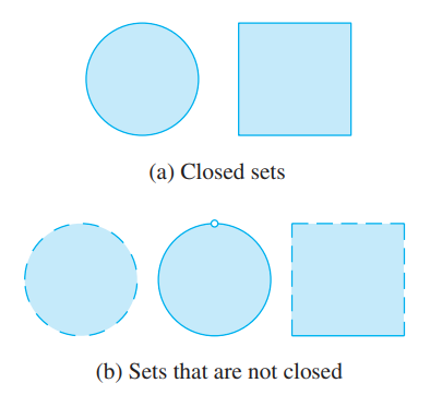
• Just as a closed interval contains its endpoints, a closed set in .$\mathbb{R}^2$ is one that contains all its boundary points.
  • For instance, the disk .$D = \{(x,y) \vert x^2 + y^2 \leq 1 \}$ is a closed set because it contains all of its boundary points (which are the points on the circle .$r = 1$)
  • But if even one point on the boundary curve were omitted, the set would not be closed
• A bounded set in .$\mathbb{R}^2$ is one that is contained within some disk – it is finite in extent

Extreme Value Theorem for Functions of Two Variables: If .$f$ is continuous on a closed, bounded set .$D$ in .$\mathbb{R}^2$, then .$f$ attains an absolute maximum value .$f(x_1, y_1)$ and an absolute minimum value .$f(x_2, y_2)$ at some points .$(x_1, y_1)$ and .$(x_2, y_2)$ in .$D$.

• If .$f$ has an extreme value at .$(x_1, y_1)$, then .$(x_1, y_1)$ is either a critical point of .$f$ or a boundary point of .$d$.
• To find the absolute maximum and minimum values of a continuous function .$f$ on a closed, bounded set .$D$:
  1. Find the values of .$f$ at the critical points of .$f$ in .$D$.
  2. Find the extreme values of .$f$ on the boundary of .$D$.
  3. The largest of the values from steps 1 and 2 is the absolute maximum value; the smallest of these values is the absolute minimum value.

14.8 Lagrange Multipliers #

• We use Lagrange Multipliers to find critical points of a surface .$f$ given some constraining surface .$g$

  Method of Lagrange Multipliers To find the maximum and minimum values of .$f(x,y,z)$ subject to the constraint .$g(x,y,z) = k$ [assuming that these extreme values exist and .$\nabla \neq 0$ on the surface .$g(x,y,z) = k$]:

  • Find all values of .$x, y, z$, and .$\lambda$ such that $$\nabla f(x,y,z) = \lambda \nabla g(x,y,z)$$ $$g(x,y,z) = k$$
  • Evaluate .$f$ at all the points .$(x, y, z)$ that result from the first step. The largest of these values is the maximum value of .$f$; the smallest is the minimum value of .$f$.

• We can decompose the first equation and use the second equation to get $$f_x = \lambda g_x;\ \ f_y = \lambda g_y;\ \ f_z = \lambda g_z;\ \ g(x,y,z) = k$$
• Notice we don’t care what .$\lambda$ is, only that it exists

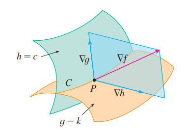
Two Constraints #

• We can use Lagrange multipliers for two constraints .$f$ and .$g$ too: $$\nabla f(x_0, y_0, z_0) = \lambda \nabla g(x_0, y_0, z_0) + \mu \nabla h(x_0, y_0, z_0)$$
• Likewise, we can decompose the equation above to get the following five equations:
  1. $$f_x = \lambda g_x + \mu h_x$$
  2. $$f_y = \lambda g_y + \mu h_y$$
  3. $$f_z = \lambda g_z + \mu h_z$$
  4. $$g(x,y,z) = k$$
  5. $$h(x,y,z) = c$$