When we manufacture many nominally “identical” components and then measure them, our measurements will inevitably show variation. Some of this variation will come from actual differences between the components’ dimensions — stemming, for example, from variation of the properties of the stock material used, cutting tool wear over time, changes in machine temperature during processing, or small, random, operator errors. Additional variation can, however, come from the measurement process itself, as there may be operator error in using a measuring instrument, or the instrument’s response may drift over time.
Ideally, we would have some way to distinguish unambiguously between measurement errors and true dimensional deviations which might take a component outside of the specified tolerance zone. In reality, however, measurement and true dimensional errors are superimposed in the reading that we obtain. The best we can do is minimize measurement errors through the use of proper technique and appropriate instrument calibration. Reducing measurement error often costs money, however, either by requiring more expensive equipment or by needing a slower, more meticulous measurement process. The measurement process used needs to be appropriate for the task at hand. As long as the measurement error is a small fraction of the tolerance zone size, it will usually suffice.
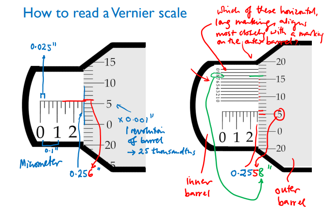
Resolution, discrimination: The smallest difference between two measurements that can be detected
E.x. in an instrument with a digital readout, the resolution corresponds to the change in reading that occurs when the least significant digit of the readout is incremented or decremented.
In an “analog” instrument, such as a micrometer with a Vernier scale, the resolution is determined by the spacing between tick marks on the finest scale on the instrument.
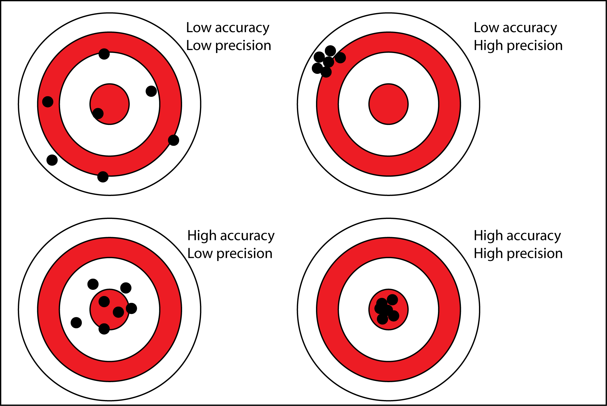
Accuracy: The amount of deviation of a measurement from the
true value (“inaccuracy” really)
Description of only
systematic errors, a measure of
statistical bias of a given measure of
central tendency; low accuracy causes a difference between a result and a true value; ISO calls this trueness
Repeatability/precision: The ability to avoid scatter/variation in successive measurements of the same physical dimension
Accuracy is the proximity of measurement results to the true value; precision is the degree to which
repeated (or
reproducible) measurements under unchanged conditions show the same results.
Given a
statistical sample or set of data points from repeated measurements of the same quantity, the sample or set can be said to be accurate if their
average is close to the true value of the quantity being measured, while the set can be said to be precise if their
standard deviation is relatively small.
Resolution, accuracy and repeatability all play a role in determining measurement error. A measurement technique could exhibit large errors in individual measurements, but when those measurements were averaged might yield a mean value that was accurate. Such a technique would have poor repeatability, and inaccurate individual measurements, but would effectively be accurate on average.
Conversely, a measurement technique might show little measurement-to-measurement variability (highly repeatable) but might always give a result that deviated greatly from the true value (highly inaccurate). Such a technique would be described as biased and would indicate poor instrument calibration.
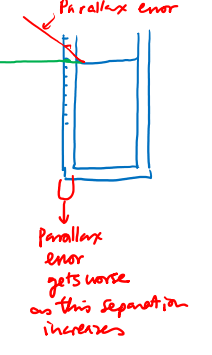
Parallax: where the scale is inadvertently held some distance from the edge being measured, and the angle of viewing affects the reading that is taken
Geometrical errors: The instrument is not aligned properly to the dimension that is to be measured.
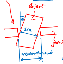
Cosine error: When failing to use the flat portions of a caliper’s jaws to ensure the axis of a cylindrical component lies perpendicular to the diameter being measured (Measurement > diameter)
Instrument/component Distortions: when the instrument is loaded excessively (e.g. pressing too hard on a caliper thumbwheel) and either the instrument or the component distorts elastically. The distortion may be invisible to the eye, but may be larger than the resolution of the measurement tool.
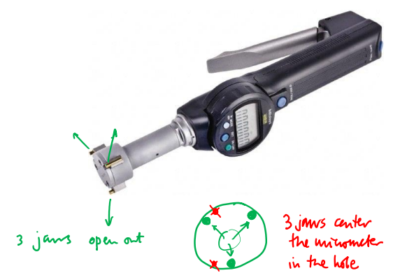
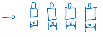
Hole gage is likely to be more accurate than calipers, because the hole gage will tend to center itself within the hole whereas the jaws of the caliper may come to rest across a chord of the hole, rather than a diameter, and thus underestimate the dimension. We thus expect caliper measurements of internal diameters to be biased towards underestimation.
Calibration errors/drift Could be due to wear of tools
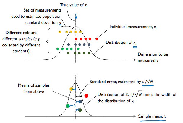
$\sigma$: Standard deviation of underlying measurement process
$\hat \sigma$: Best estimate of standard deviation of the process, based on $N$ measurements of it:
$$\hat \sigma = \sqrt{\frac{\sum_{i=1}^N (x_i - \hat x)^2}{N-1}}$$
The mean of our $N$ values will not exactly equal the true value.
But if the measurement process is centered on the true value, the mean of $N$ measurements follows a normal distribution with standard deviation $\sigma / \sqrt N$ –
central limit theorem
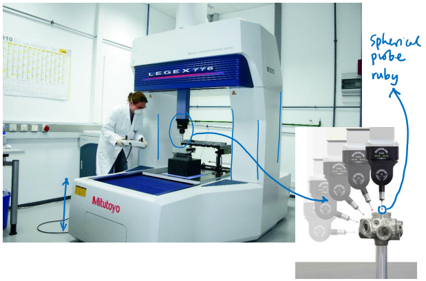
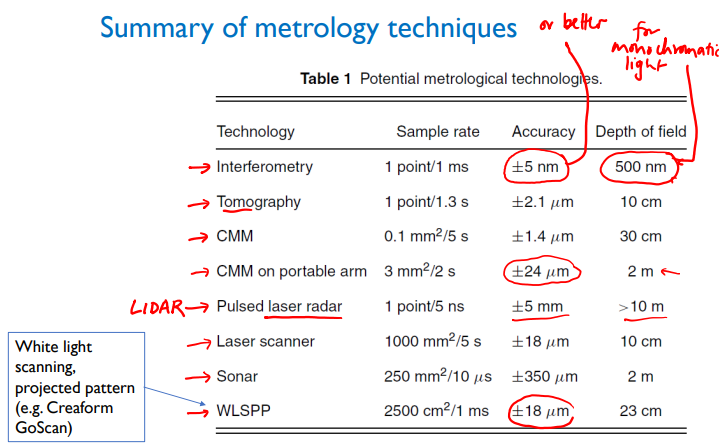
Industrial dimensional measurement has increasingly moved towards automated coordinate measurement machines (CMMs). A CMM has a solid probe mounted in a rigid frame and its position is actuated with motors and leadscrews having highly accurate positional feedback. In sophisticated machines, the probe may have five or more degrees of freedom to enable access to complex geometries. The probe is touched against multiple locations on a component under test, contact is detected by force sensors in the probe assembly, and software interprets the measurements to check dimensions against a solid model.
The probe is usually spherical and made of a hard material with a low friction coefficient such as synthetic ruby, to enable many measurements to be made without the tip significantly eroding or visibly scratching the component under test.
Lower-cost CMM machines are available, which are not as rigid but are more portable. These usually have the probe assembly on an articulated arm, with encoders in each joint that determine angular positions of the joints and thus the position of the tip at any given moment. We will see a demonstration of such an arm, a Romer system from Hexagon Metrology, in Lab 7on dimensional measurements. The accuracy of an arm-mounted CMM may be more than ten times poorer than a conventional, more rigid frame-mounted system.
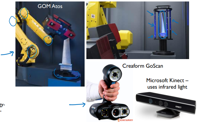
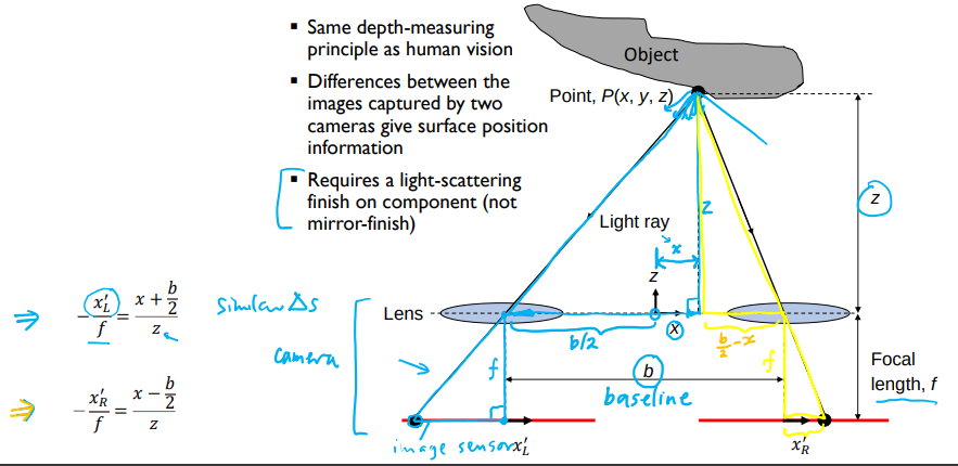
Stereo vision systems use the same principle as human sight to extract depth information from pairs of images. By illuminating a component with structured light to define unambiguous features on a surface, and then sweeping a pair of cameras around the component, software can determine complex 3D shapes which would require hours of laborious mechanical scanning to measure with a CMM.
They require the surface being measured to scatter light uniformly, so polished surfaces have to be laboriously coated with a thin layer of fine powder – which must later be removed. This requirement removes some of the advantages over traditional CMMs. There is a basic tradeoff between dimensional resolution and field of view, and there is debate about how well the accuracy of these systems has been characterized.
A different type of optical metrology exploits the wave properties of light to make dimensional measurements with a resolution smaller than a single wavelength. This technique has seen wide deployment, for example, in measuring sub-micrometer structures on integrated circuits, and characterizing finely polished mirrors, lenses and prisms.
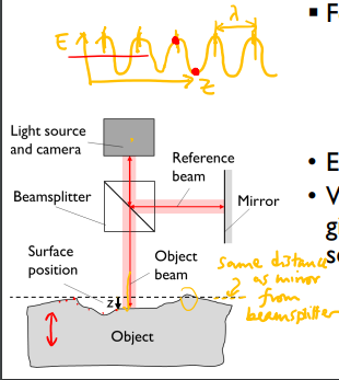
In optical interferometry as shown in the class, a beam of light is split by a semi-mirrored surface (beamsplitter). One of the resulting beams (the reference beam) reflects off a flat mirror and back towards an image sensor. The other beam (object beam) is directed down to the sample surface, and then back up to the image sensor.
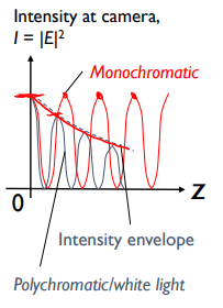
Let us first consider monochromatic (single-wavelength) light. When the distance travelled by the object beam is an odd number of half wavelengths greater or less than that travelled by the reference beam, the beams destructively interfere at the image sensor and yield a dark signal at a particular pixel. When the path length difference is an even number of half wavelengths, there is constructive interference and a bright signal. For intermediate path length differences, there is an intermediate signal. Each pixel in the image sensor picks up light from a different location on the sample object, and at any given instant will receive different interference intensities if the object is not perfectly smooth. The object being measured is slowly scanned vertically away from the beamsplitter, and as the path lengths change, the signals at the image sensor oscillate. With monochromatic light, however, these oscillations are periodic and the relative positions of adjacent portions of the surface cannot be unambiguously determined, especially if the surface roughness is more than about a quarter of a wavelength.
Thus, white light is more commonly used. Here, the effects of the many wavelengths superimpose on a grayscale image sensor, and the interference intensity is at its peak only when the path length difference between object and reference beams is exactly zero. As the path length differences change, the intensity oscillations decay in magnitude, and software can fit an envelope to these intensity variations to establish relative surface positions.
This technique is suitable for highly accurate and precise measurements of sub-micrometer dimensional variations, but is typically limited to fields of view of a few millimeters. Moreover, because it relies on reflections, surfaces must be reasonably flat; otherwise the reflected light would not bounce back towards the image sensor.