02-08: Matrix Transformations #
Linear Transformations #
- Linear Transformation: In the previous practice set, we discussed the idea of a matrix .$A^{M \times N}$ as a linear transformation.
- Effectively, in the equation .$A \vec x = \vec b$, the matrix itself can be considered a transformation .$f : \mathbb{R}^{N} \to \mathbb{R}^{M}$ which takes a vector .$\vec x^{N \times 1}$ of inputs and returns a vector .$\vec b^{M \times 1}$ of outputs
- That is, matrices are operators that transform vectors
- Effectively, in the equation .$A \vec x = \vec b$, the matrix itself can be considered a transformation .$f : \mathbb{R}^{N} \to \mathbb{R}^{M}$ which takes a vector .$\vec x^{N \times 1}$ of inputs and returns a vector .$\vec b^{M \times 1}$ of outputs
- Just as .$f$ is a linear transformation iff homogeneity and super position hold, matrix-vector multiplications satisfy linear transformation:
$$A \cdot (\alpha \vec x) = \alpha A \vec x$$ $$A \cdot (\vec x + \vec y) = A \vec x + A \vec y $$
State Transformation #
- As such, we can think about matrices as state transformations;
- If we have a list of inputs representing some current state at some timestep .$n$ (given by .$\vec x(n)$), then when a matrix .$A$ operates on that state, it transforms it into a new state at the next time step (.$\vec x(n + 1)$).
- Consider a timestep to be a very small unit of time. Our systems here will be discrete, meaning that the transition of water happens exactly at each timestep, and not between timesteps
- Aside: But in reality, water is flowing continuously! To model this rigorously, we need linear differential equations, but for now, if the timestep we take is very small, the discrete model is quite good as an approximation.
- Example: Water Pulps (
Note5 )
- At each time step, some portion of the water in each pump goes to itself, and some portion goes to each of the other pumps. The general state transition matrix formula for an .$n$-state system (assuming the initial and final state vectors have the same length .$n$) is as follows:
$$ \begin{bmatrix} \vec P_{1 \to \dots} & \vec P_{2 \to \dots} & \dots & \vec P_{N \to \dots} \\ \end{bmatrix}$$ $$\equiv$$ $$\begin{bmatrix} P_{1 \to 1} & P_{2 \to 1} & … & P_{N \to 1}\\ P_{1 \to 2} & P_{2 \to 2} & … & P_{N \to 2}\\ \vdots & \vdots & \ddots & \vdots\\ P_{1 \to N} & P_{2 \to N} & … & P_{N \to N} \end{bmatrix} $$
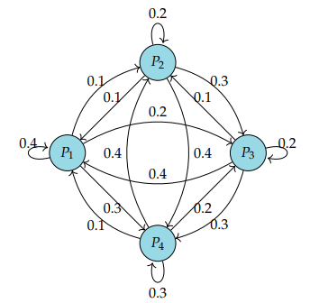 $$\begin{bmatrix}
0.4 & 0.1 & 0.4 & 0.1\\
0.1 & 0.2 & 0.1 & 0.4\\
0.2 & 0.3 & 0.2 & 0.2\\
0.3 & 0.4 & 0.3 & 0.3
\end{bmatrix}$$
$$\begin{bmatrix}
0.4 & 0.1 & 0.4 & 0.1\\
0.1 & 0.2 & 0.1 & 0.4\\
0.2 & 0.3 & 0.2 & 0.2\\
0.3 & 0.4 & 0.3 & 0.3
\end{bmatrix}$$- Notice that all of the water goes somewhere and none comes up out of thin air; that is, the water is a conserved quantity. We don’t have any leakage or generation of water in the system.
- This isn’t always true, but the idea of conservation will largely hold true, especially for systems based in physical reality.
- We can tell if the transformation is conservative by looking at each column’s values describe the movement of water from a specific node to other nodes. If any column’s values do not sum to exactly 1, then something is being lost or created in the system as a whole.
- In addition, if a specific column’s sum is greater than 1, matter is entering the system through that node; conversely, if a specific column sum is less than 1, matter is leaving the system through that node.
- Recognize that, given information about only a single node’s column sum, we can never definitely say if the overall system is conservative or not; we only know if it might be conservative, based on other nodes.
- Diagram .$\to$ Matrix:
- Given a state transition diagram, we can create the corresponding state transition matrix by reading the values at each arrow, noting the directionality (these are directed edges) and populating the rows one by one.
- Similarly, given a matrix, we can draw the appropriate number of nodes and label arrows going to/from each node with the values as indicated by the matrix.
- How do we go back in time?
- That is, we want some transition matrix .$B$ such that .$\vec x (t-1) = B \vec x(t)$
- Flipping the direction of the edges won’t work…
- Transpose won’t either…
- Which leads us to…
02-10: Inverse #
Matrix Inverse #
- Purpose
- We know that .$\vec x(t+1) = Q \vec x (t)$ and want some reverse-matrix .$P$ such that .$\vec x (t) = P \vec x (t+1)$
$$P \vec x(t+1) = PQ\vec x(t)$$ $$P \vec x(t+1) = I \vec x(t)$$
$$\vec x(t+1) = Q \vec x(t)$$ $$\vec x(t+1) = Q(P \vec x(t+1))$$ $$\vec x(t+1) = I \vec x(t+1)$$
- We know that .$\vec x(t+1) = Q \vec x (t)$ and want some reverse-matrix .$P$ such that .$\vec x (t) = P \vec x (t+1)$
- Consider .$A$ as an operator on any vector .$\vec x \in \mathbb{R}^{n}$:
- What does it mean for .$A$ to have an inverse? It suggests that we can find a matrix that “undoes” the effect of matrix .$A$ operating on any vector .$\vec x \in \mathbb{R}^{n}$. What property should .$A$ have in order for this to be possible?
- A should map any two distinct vectors to distinct vectors in .$ \mathbb{R}^{n}$, i.e., .$A \vec x_1 \neq A \vec x_2$ for vectors .$\vec x_1, \vec x_2$ such that .$\vec x_1 \neq \vec x_2$.
- Definition: Let .$P, Q \in \mathbb{R}^{N \times N}$ be square matrices (we tackle non-square in 16B)
- .$P$ is the inverse of .$Q$ if .$PQ = QP = I$
- We say .$P = Q^{-1}$ and .$Q = P^{-1}$
- Steps to solve with Gaussian Elimination are shown on
slide 50 or ‘more’ formally in
Notes 6, page 3
- For any .$n \times n$ matrix .$M$, we can perform Gaussian elimination on the augmented matrix:
- If at termination of Gaussian elimination, we end up with an identity matrix on the left, then the matrix on the right is the inverse of the matrix .$M$
- If we don’t end up with an identity matrix on the left, we will have a row of zeros, (which indicates that the rows of .$M$ are linearly dependent) and that the matrix is not invertible
$$\begin{bmatrix} & & | & & \\ & M & | & I_n & \\ & & | & & \\ \end{bmatrix} $$
$$ \begin{bmatrix} & & | & & \\ & I_n & | & M^{-1} & \\ & & | & & \\ \end{bmatrix}$$
Inverse of a 2x2 matrix #
- You can derive this via Gaussian elimination (flip .$a$ with .$d$, negate .$b$ and .$c$, then divide by .$ad-bc$)
$$A = \begin{bmatrix} a & b\\ c & d\\ \end{bmatrix}$$
$$A^{-1} = \frac{1}{ad-bc} \begin{bmatrix} d & -b\\ -c & a\\ \end{bmatrix}$$
- .$ad-bc$ is the determinant, so we can check quickly if an inverse exists for a square matrix by checking if they determinant exists
- See slide 8
- Determinant is the area the vectors form. So if they vectors form some zero-area (or volume in 3D) then it’s not one-to-one and thus not invertible
Theorems #
Theorem Note 6.1 #
If .$A$ is an invertible matrix, then its inverse must be unique
- Suppose .$B_1, B_2$ are both inverses of the matrix .$A$. Then we have
- Notice that by associativity of matrix multiplication, the left hand side of the equation above becomes
- We see that .$B_1 = B_2$, so the inverse of any invertible matrix is unique.
$$AB_1 = B_1 A = I$$ $$AB_2 = B_2 A = I$$
$$AB_1 = I \Longrightarrow B_2(AB_1) = B_2 I = B_2$$ $$B_2 (AB_1) = (B_2 A)B_1 = IB_1 = B_1$$ $$\therefore B_1 = B_2$$
- Another important property of inverses is that the “left” inverse and the “right” inverse are equal to each other. In particular…
Theorem Note 6.2 #
If .$QP = I$ and .$RQ = I$, then .$P = R$. The matrix .$P$ can be thought of as the “right” inverse of .$Q$ and the matrix .$R$ can be thought of as the “left” inverse of .$Q$.
- We start the proof by noticing that we know two things .$QP = I$ and .$RQ = I$. To move ahead, we can try setting .$QP = RQ$, but we cannot proceed from here, since the multiplication by .$Q$ is on different sides. So instead we take the equation .$QP = I$ and multiply both sides on the left by .$R$. This gives $$R(QP) = R(I) = R$$
- Now, using the associative property of matrix multiplication we have that $$R(QP) + (RQ)P = IP = P$$
- Here we used .$RQ = I$. Combining these two equations, we have that .$R = P$, and we are done
Theorem Note 6.3 #
If a matrix A is invertible, there exists a unique solution to the equation .$A \vec x = \vec b$ for all possible vectors .$\vec b$.
- Let’s try to prove this. To do so, we need to prove two statements:
- That there exists at least one solution to the equation .$A \vec x = \vec b$, and that
- There exists no more than one solution to the equation .$A \vec x = \vec b$.
- For both of the above statements, .$\vec b$ can be any vector in .$\mathbb{R}^{n}$
- Let’s prove the first statement first. Imagine we are given a vector .$\vec b$. Consider the candidate solution .$\vec x = A^{−1} \vec b$. Observe that $$A \vec x = A(A^{-1} \vec b) = (AA^{-1}) \vec b = \vec b$$
- Thus, our candidate solution satisfies the equation .$A \vec x = \vec b$, so there exists at least one solution to that equation!
- Now, let’s show the second statement – that no more than one solution to the equation .$A \vec x = \vec b$ can exist. Consider a particular solution .$\vec x$, so .$A \vec x = \vec b$. Pre-multiplying both sides of this equation by .$A^{−1}$, we obtain $$A^{-1}(A \vec x) = A^{-1} \vec b \Longrightarrow \vec x = A^{-1} \vec b$$
- Therefore, if .$\vec x$ exists, it must be the particular vector .$A^{−1} \vec b$. In other words, there exists at most one solution to the equation .$A \vec x = \vec b$, so we have proven the second statement
Theorem Note 6.4 #
If a matrix .$A$ is invertible, its columns are linearly independent.
- Let’s prove this theorem. We know that the statement “the columns of .$A$ are linearly independent” is equivalent to the statement “.$A \vec x = \vec 0$ only when .$ \vec x = \vec 0$.” This fact follows from the definition of linear independence: by definition, if .$\vec v_1, \dots, \vec v_n$ are linearly independent, then .$\sum_{i=1}^n x_i \vec v_i$ is only .$\vec 0$ when .$x_i = 0$.
- Using the column perspective of matrix multiplication (covered in Note 3), .$A \vec x = \sum_{i=1}^n x_i \vec v_i$ where .$\vec v_i$ is the .$i$th column of .$A$. Therefore, .$A \vec x = \vec 0$ only when all .$x_i = 0$.
- Therefore, we can rephrase what we’re trying to prove as $$A^{-1} \text{ exists } \Longrightarrow A \vec x = \vec 0 \text{ only when } \vec x = \vec 0$$
- To prove this, assume that .$A$ is invertible. Let .$\vec v$ be some vector such that .$A \vec x = \vec 0$: $$A \vec x = \vec 0 \text{ left-multiply by } A^{-1}$$ $$A^{-1} A \vec v = I \vec v = \vec 0$$ $$\vec v = \vec 0$$
Theorem Lecture #
.$A$ is invertible, iff the columns of are linearly independent.
- That is,
- If columns of .$A$ are liner dependent then .$A^{-1}$ does not exist
- If .$A^{-1}$ exists, then the cols. of .$A$ are linearly independent
- Proof concept: Assume linear dependence and invertibility and show that it is a contradiction
- From linear dependence: .$\exists \vec \alpha \neq 0$ such that .$A \vec \alpha = 0$:
- But .$\vec \alpha \neq 0$, hence, .$A^{-1}$ DNE
$$A \vec \alpha = 0$$ $$A^{-1} A \vec \alpha = A^{-1} 0$$ $$I \vec \alpha = 0$$
- Thus, the following statements are equivalent:
- Matrix .$A$ is invertible
- .$A$ has linearly independent columns
- .$A$ is full rank
- .$A \vec x = \vec b$ has a unique solution
- .$A$ has a trivial nullspace
- The determinant of is not zero