21.1 Static Electricity; Electric Charge and its Conservation #
- “Charged” objects posses a net electric charge
- Unlike charges attract; like charges repel
- Charges on glass are positive, charges on plastic is negative
- Law of Conservation of Electric Charge:
- Whenever a certain amount of charge is produced in one object, an equal amount of the opposite type of charge is produced in another object
- Charges cannot be destroyed or created
- E.x. a plastic ruler is rubbed with a paper towel. The plastic acquires a negative charge and the towel obtains an equal positive charge
- In other words, the net amount of electric charge produced in any process is zero: .$\Sigma Q = 0$
- Whenever a certain amount of charge is produced in one object, an equal amount of the opposite type of charge is produced in another object
21.2 Electric Charge in the Atom #
- Atoms are made up of positive nucleus surrounded by at least one negatively charged electron.
- Inside the nucleus are protons which are positively charged and neutrons which have no charge
- The charges of electrons and protons are equal in magnitude
- E.x. neutral atoms with no charge contain an equal number of protons and electrons
- When an atom gains a charge (by losing/gaining electrons), it then has a net charge and is called an ion
- Neutral objects have a net charge of zero
- Over time, objects left alone with a charge tend to lose their charge
- This is because over time, electrons are exchanged with water molecules in the air
- Water molecules are polar: They are neutral, their charges aren’t equally distributed
- Thus, on rainy days it’s harder for an object to maintain a charge for too long
21.3 Insulators and Conductors #
- Conductor: Material that allow charge to flow between objects
- Metals tend to be good conductors
- Electrons (charges) are relatively lose: can move freely within metal, but can’t leave easily
- Called free or conduction electrons
- Insulator: Opposite of conductors; don’t easily allow a flow of charge
- Most materials other than metals tend to be good insulators
- Notably rubber and wood
- Electrons are bound very tightly to the nuclei
- Almost no free electrons
- Most materials other than metals tend to be good insulators
- Semiconductors: Somewhere between the two former
- Silicon, germanium
- Less free electrons than a conductor, but more than an insulator
21.4 Induced Charge; Electroscope #
- Conduction: Charge transfer by physical contact
- E.x. a positively charged metal rod touches a neutral metal rod. Free electrons from the neutral rod will then flow (transfer) to the charged rod, leaving the formerly neutral rod now slightly positively charged
- Induction: Charge distribution altered by bringing two objects close, but not touching
- Unlike conduction, induction doesn’t alter the net charge of objects when the inducer is taken away
- However, induction can redistribute the existing charges on the induced object
- Grounded Objects
- Objects can be ground to the earth with a conducting wire
- The earth is very large and can conduct, so it easily accepts/gives up electrons
- Therefore, when an object is induced by another charged object, the original objects will become charged
- If the wire is ever cut when the object is under induction, the charge will stay in the object
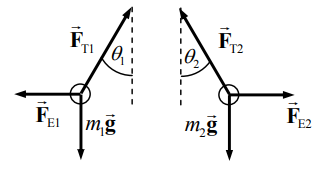
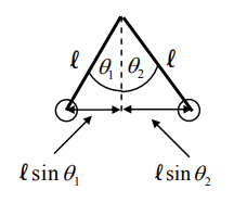
- Electroscope
- .$\vec F \propto \text{angle of deflection}$
- .$y$-axis: .$F_{T1} \sin \theta_1 = F_{21}$
- .$x$-axis: .$F_{T1} \cos \theta_0 = m_1 g$
- .$F_{21} = m_1 g \tan \theta_1 \approx m_1 g \theta_1$
- .$F_{21} = - F_{12}$ ( Newton’s Third) .$ \Longrightarrow \theta_1/\theta_2 = m_2/m_1$
- .$d = l (\theta_1 + \theta_2)$
21.5 Coulomb’s Law #
Coulomb’s Law: $$E_\text{source} = k \frac{Q_\text{source}}{r^2} \Longrightarrow F = EQ = \bigg(k \frac{Q_1}{r^2}\bigg) (Q_2) = k\frac{Q_1 Q_2}{r^2}$$ where .$k$ is a constant equal to .$\frac{1}{4\pi\varepsilon_0} = 8.988 \cdot 10^9 \text{ N m$^2$/C$^2$}$
- Very similar to
universal gravitation equation
- However…
- .$F_C$ can repel, whereas .$F_G$ is always attractive
- .$F_C$ only acts on charged objects, whereas .$F_G$ acts on neutral objects too
- .$F_G/F_C \approx 10^{-40} \Longrightarrow F_C \gg F_G$
- However…
- The coulomb (.$\text{C}$) is the SI unit for charge
- Properties of Coulomb Force:
- It can be attractive and repulsive
- It is not a contact force
- Inversely proportional to .$r^2$
- Proportional to amount of charge .$Q$
- The smallest charge we’ve observed is the elementary charge: .$e = 1.6022 \cdot 10^{-19} \text{ C}$
- Electrons have a charge equal to .$-e$
- Protons have a charge equal to .$+e = -Q_\text{electron}$
- Charges are Quantized
- That is, all charges are multiples of .$e$
- Since electrons are elementary particles, by definition they can’t be divided.
- .$k$ can also be written as .$\frac{1}{4\pi\varepsilon_0}$
- .$\varepsilon_0$ is called the permittivity of free space
- .$\varepsilon_0 = \frac{1}{4\pi k} = 8.85 \cdot 10^{-12} \text{C$^2$/N m$^2$}$
21.6 Electric Field #
- Electric fields extend outward from every charge and permeates all of space
$$\overrightarrow E = \lim_{q\to0}\frac{\overrightarrow F}{q} \Longrightarrow \overrightarrow F = q \overrightarrow E$$
- .$q$ is a positive charge
- .$\overrightarrow F$ is the forces the field exserts on .$q$
- Has units newtons per coulomb (.$\text{N/C}$)
- We can combine this with Coulomb’s law to get
$$\overrightarrow E = \frac{kqQ/r^2}{q} = k \frac{Q}{r^2} = \frac{1}{4\pi\varepsilon_0} \frac{Q}{r^2}$$
- We see that .$\overrightarrow E$ is independent of the non-source particle .$q$
- .$Q$ is the particle that is responsible for the field in the first place
- An electric field at a given point is the sum of all other electric fields that act on that point $$\overrightarrow E = \overrightarrow E_1 + \overrightarrow E_2 + …$$
21.7 Electric Field Calculations for Continuous Charge Distributions #
- We can extend our previous definition to calculus as
$$\overrightarrow E = \int d \overrightarrow E = k \int \frac{1}{r^2}\ dq = \frac{1}{4\pi\varepsilon_0} \int \frac{1}{r^2}\ dq$$
- .$dq = \lambda\ dl \text{ (line)} = \sigma\ dA \text{ (disk)} = \rho\ dV \text{ (sphere)}$
Calculating field generated by a continuous charge distribution
- Draw an arbitrary “piece” of charge distribution; don’t choose a special point such as the end or exact middle. The piece should be infinitesimally long and/or wide. Thus, its length or width will be something like .$dx$ or .$ds$
- Write an expression for .$dq$, the corresponding infinitesimal charge of that piece in terms of .$dx$ or .$ds$ or whatever. Recall .$dq = \frac{\text{total charge}}{\text{total length}} \times \text{(tiny length of piece)}$
- Using Coulomb’s law, find the infinitesimal electric field at that point of interest (e.x. some point .$P$) generated by the piece chosen in step 1. When necessary, break .$d\vec E$ into components, .$dE_x$ and .$dE_y$
- Integrate .$dE_x$ or .$dE_y$ over the whole charge distribution to obtain the total electric field in the .$x$ or .$y$ direction respectively
- When solving problems, it’s a good idea to use symmetry, check charge direction, and (when applicable) use bounds of .$r \in [0, \infty]$
- We can write equation for an infinite plane holding a uniform surface charge density .$\sigma$
$$2A \cdot \overrightarrow E = \frac{\sigma A}{\varepsilon_0} \Longrightarrow \overrightarrow E = \frac{\sigma}{2\varepsilon_0}$$
- This also applies in the case where a charge is close to an infinite surface (so that the distance to the surface is much greater than the distance to the edges)
- In the case where there are two oppositely charged sheets parallel to one another, the field is .$\vec E = \frac{\sigma}{\varepsilon_0}$ since there are two charges creating the field
- The case involving an infinitely long wire can be written generally as
$$\overrightarrow E \cdot 2\pi RL = \frac{\lambda L}{\varepsilon_0} \Longrightarrow \overrightarrow E = \frac{\lambda}{2\pi\varepsilon_0 \cdot r}$$
- .$r$ is the distance from a particle to the wire
21.8 Field Lines #
- To visualize electric fields, we draw electric field lines or lines of force
- Three properties of Electric Field Lines:
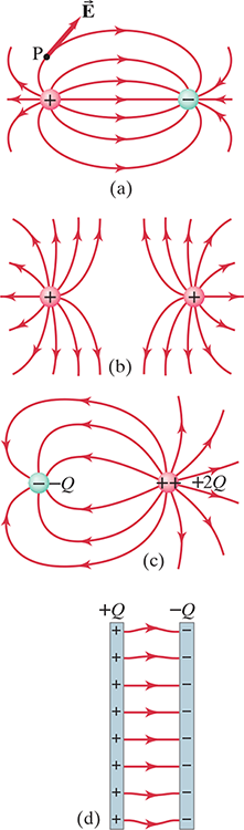
- Electric field lines indicate the direction of the electric field; the field points are in the direction tangent to the field line at any point – see point .$P$ in .$\text{(a)}$
- The lines are drawn so that the magnitude of the electric field, .$E$, is proportional to the number of lines crossing unit area perpendicular to the lines (i.e. a circle ‘hugging’ a point charge). The closer together the lines, the stronger the field.
- Electric field lines start on positive charges and end on negative charges; and the number starting or ending is proportional to the magnitude of the charge.
- .$\text{Density} = \frac{\text{number of lines crossing surface}}{\text{area surface}}$
- .$\text{1 Coulomb} = \frac{1}{\varepsilon_0} \cdot \text{ lines}$
- .$\therefore \text{Density} = \frac{q}{\varepsilon_0 4\pi r^2} \Longrightarrow \vec E$
- In the case of two oppositely charged parallel & equally spaces plates – such as case .$\text{(d)}$ – we can write the field as
$$\overrightarrow E =\text{const.} = \frac{\sigma}{\varepsilon_0}=\frac{Q}{\varepsilon_0 A}$$
- .$Q =\sigma A$ is the charge on one plate of area .$A$
- Field lines never cross because it wouldn’t make sense for an electric field to have two directions at the same point.
Electric Dipole #
- A combination of two equal but opposite charges next to one another – see .$(\text{a})$ above
- Dipole Moment is when represented by vector .$\vec{p}$ of magnitude .$Ql$
- Molecules that have dipole moments are called polar molecules
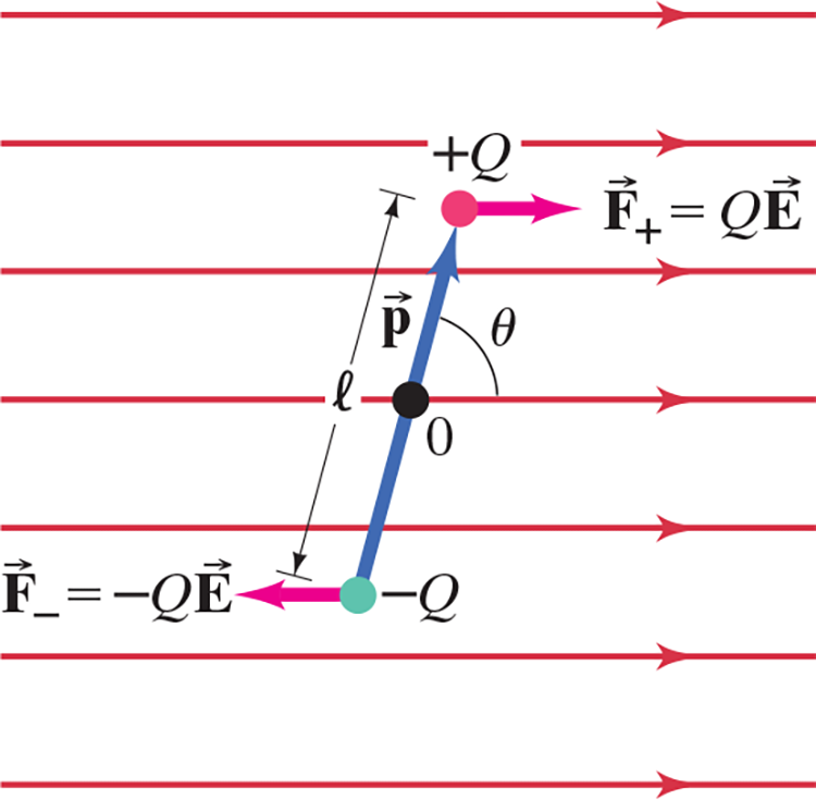
- A dipole in a uniform electric field feels no net force, but does have a net torque (unless .$\vec p \parallel \vec E$)
- If .$\vec p \not \parallel \vec E$, .$W =\int_{\theta_1}^{\theta_2} \tau d\theta$ where .$\tau = -\vec p\vec E\sin\theta = \vec p \times \vec E$
- Simplifies to .$W =\vec p\vec E(\cos\theta_2 - \cos\theta_1)$
- Thus, work/torque is most at .$\theta = 90^\circ$ or .$180^\circ$ depending on .$\vec E$ direction
- Pay attention to right hand rule when solving
- If .$r \gg l \Longrightarrow \overrightarrow E \propto 1/r^3$
21.9 Electric Fields and Conductors #
- The static electric field inside a conductor is zero (in static situations where electrons have had time to stop moving)
- For that reason, any net charge on a conductor distributes itself on the surface
- Charges inside conductors act as if the conductor isn’t there
- All the electric field lines just outside a charged conductor are perpendicular to the surface
21.10 Motion of Charged Particle #
- Vector Form of Forces
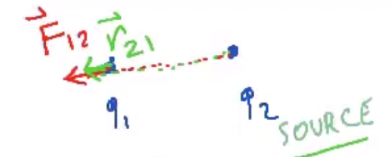
$$\overrightarrow F_{12} = k \frac{q_1 q_2}{r^2} \cdot \widehat r_{21}$$
- Notation:
- .$\overrightarrow F_{12}$ means force on .$q_1$ by .$q_2$ since .$q_2$ is the source charge
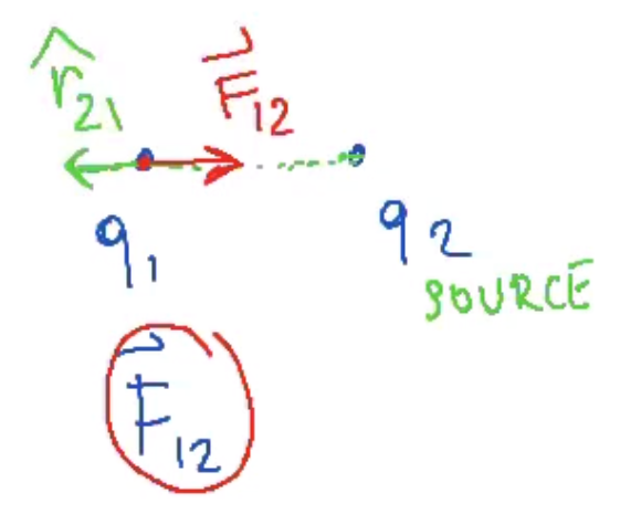
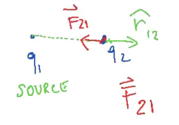
- .$\widehat r_{21} = - \widehat r_{12} \Longrightarrow \overrightarrow F_{12} = -\overrightarrow F_{21}$
- Direction
- If .$q_1 q_2 > 0$ (same sign, repulse), then the force and unitary vectors both point away from the two charges
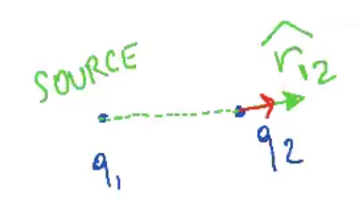
- If .$q_1 q_2 > 0$ (same sign, repulse), then the force and unitary vectors both point away from the two charges
- Notation:
- If .$q_1 q_2 < 0$ (opposite sign, attract), then the force vector points towards the two charges and the unitary direction vector still points away from the two charges
- Superposition Principle
- In a system considering multiple (3+) charges, forces acting on .$q_1$ by .$q_2$ (.$F_{12}$) is independent from whether other charges are present
- Total forces acting on .$Q_1$ can be written as .$\overrightarrow F = \overrightarrow F_{12} + \overrightarrow F_{13} + \dots$
- Remember to break down the vectors into .$x/y$ components when adding them
- E.x. .$F_{1x} = F_{12x} + F_{13x} + \dots$
- Realize that the axis are arbitrary
- Remember to break down the vectors into .$x/y$ components when adding them
- .$\theta = \tan^{-1}\Big(\frac{F_x}{F_y}\Big)$
- Charges in Fields
- Charge moving with .$\vec v$ that is parallel to uniform field .$\overrightarrow E$
- .$\overrightarrow F = q \overrightarrow E = m \vec a \Longrightarrow a_x = \frac{q}{m}\overrightarrow E = \text{const.}$
- .$\vec v = \sqrt{2a_x \vec d} = \sqrt{\frac{2q}{m}\overrightarrow E_x \vec d}$
- Charge moving with .$\vec v$ that is orthogonal to uniform field .$\overrightarrow E$
- Similar to projectile in gravitational field: .$\vec g \sim \overrightarrow E$
- .$\overrightarrow F_x = 0 \Longrightarrow v_{x2} = v_{x1};\ \ a_x = 0$
- .$\overrightarrow F_y = q \overrightarrow E = m a_y;\ \ a_y = \vec a = \frac{q}{m}\overrightarrow E = \text{const.}$
- .$y(t) = \frac{1}{2} \frac{q\overrightarrow E}{m}t^2$
- Charge moving with .$\vec v$ that is parallel to uniform field .$\overrightarrow E$
21.11 Electric Dipoles #
- Notes for this chapter are under 21.8 – Electric Dipole