01-18: Course Introduction #
All logistics, no notes!
01-20: Introduction to Imaging, Tomography, and Linear Equations #
System Design #
- We use devices, such as imagers, that provide information, such as a visual representation of a system
- Often, these devices don’t work alone – they are part of a larger system that uses a combination of both physical sensors and signal processing techniques.
- When we take projections of images, we tend to need to take multiple measuring (pictures) from differing angles
- Otherwise we have issues with overlap and ambiguity
- To generate 3D models, we need these multiple perspectives
- We ideally want to design a system that gives us a set of linear equations
- Some times we can only approximate these linear equations
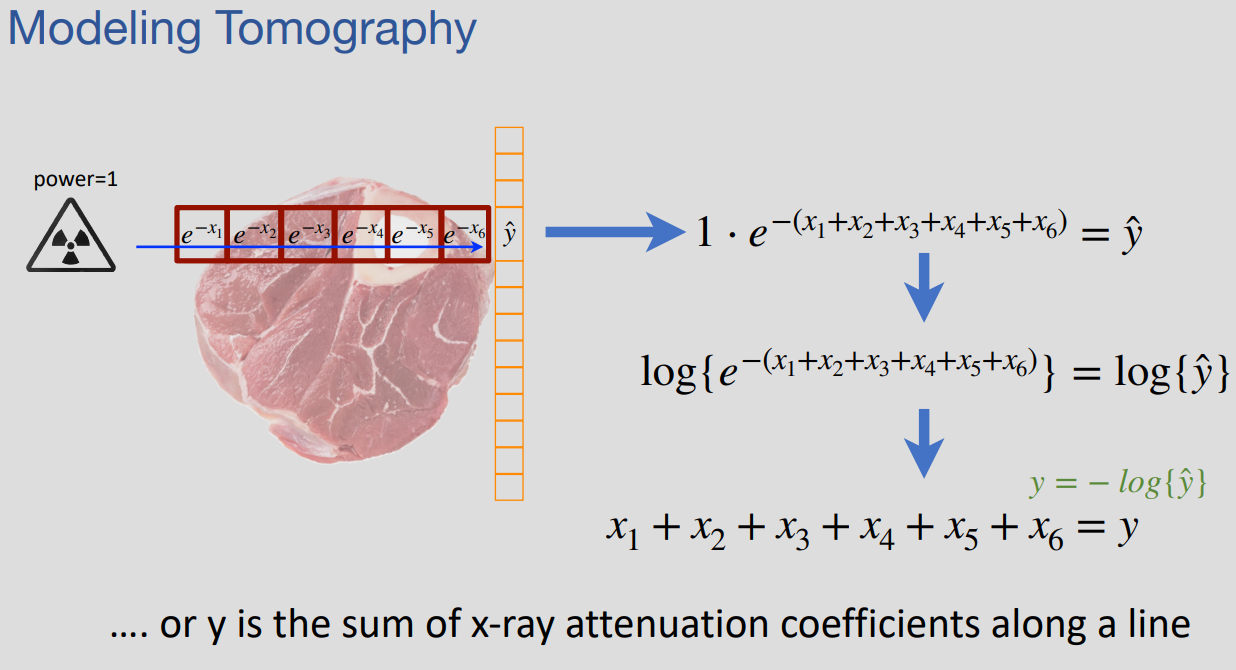
- Lots of physical processes (i.e xrays!) are exponential so we just slap a log on it
- .$\hat y = p \cdot (e^{x_1} + \dots + e^{x_n})$
- .$y = -\log_e (\hat y \cdot p^{-1}) = x_1 + \dots + x_n$
- .$\hat y$ is our measured energy value
- .$x_n$ is the .$n$th ‘pixel’
- .$p$ is the power of the energy source
Tomography Example
- To solve, we need enough independent equations that do not contain redundant information, otherwise there will be multiple ambiguous solutions
- Different models are made up of different configurations (of the energy source and measuring sensor) and result in different system of equations
- We can obtain equations by moving both the energy source and measuring sensor (think document scanner) to get each individual pixel
- We can also move the energy source alone instead – think camera pointed at image with a projector used to light up certain (group of) pixel(s)
- Different patterns have pros/cons – speed, resolution, accuracy, number of measurements, energy use
Linear Algebra #
- The study of linear functions and linear equations, typically using vectors and matrices
- Linearity is not always applicable, but can be a good first-order approximation
- There exist good fast algorithms to solve these problems (and lots of fun properties!)
- Consider .$f(x_1, \dots, x_n) : \mathbb{R}^n \to \mathbb{R}$; .$f$ is linear if the following hold…
- Homogeneity: .$f (\alpha x_1, \dots, \alpha x_n) = \alpha f(x_1, \dots, x_n)$
- If I scale the input by a scalar (i.e. by a factor of 2) then the output should also scale by the same factor
- Super position (distributivity): if .$x_i = y_i + z_i$ then .$f(y_1 + z_1, \dots, y_n + z_n) = f(y_1, \dots y_n) + f(z_1, \dots z_n)$
- 2 possible inputs:
- Pass the first input through the system to get a value.
- Pass another input through the system, and get another value.
- Add those two values to get a result.
- 1 possible input:
- Pass the summation of value 1 and value 2 through the system to get a result.
- If the result of both approaches are equal, then distributivity holds. Otherwise, distributivity does not hold.
We can account for both Homogeneity and Super position by proving the function holds under the following equation: $$\alpha_1 f(x_1, \dots x_n) + \dots + \alpha_n f(y_1, \dots, y_n) = f(\alpha_1 x_1 +\alpha_n y_1, \dots, \alpha_1 x_n + \alpha_n y_n)$$ where .$y_n$ is a some scalar
- 2 possible inputs:
- Homogeneity: .$f (\alpha x_1, \dots, \alpha x_n) = \alpha f(x_1, \dots, x_n)$
- Linear functions can always be expressed as .$f(x_1, \dots, x_n) = c_1 x_1 + \dots + c_n x_n$
- For .$\mathbb{R}^2$, that is, .$f(x_1, x_2) = c_1 x_1 + c_2 x_2$
- We know this system is linear so it follows these two rules above. So we should set up an equation where we can apply these properties.
$$\begin{align} x_1 &= 1 \cdot x_1 + 0 \cdot x_2;\ &x_2 = 0 \cdot x_1 + 1 \cdot x_2 \\ \text{Let}\quad y_1 &= 1, z_1 = 0; &y_2 = 0, z_2 = 1 \\ \Longrightarrow x_1 &= x_1 y_1 + x_1 z_1;\ &x_2 = x_2 y_2 + x_2 z_2 \\ \Longrightarrow x_1 &= x_1 (y_1 + z_1);\ &x_2 = x_2 (y_2 + z_2) \end{align}$$ $$\begin{align} \text{Therefore, } f(x_1, x_2) &= f(x_1 y_1 + x_2 z_1, x_1 y_2 + x_2 z_2) \\ &= x_1f(y_1, y_2) + x_2f(z_1, z_2) \\ &= x_1f(1, 0) + x_2f(0, 1) \\ &= c_1 x_1 + c_2 x_2\ \blacksquare \end{align}$$
- Linear Set of Equations
Consider the set of .$M$ linear equations with .$N$ variables: $$\begin{matrix}a_{11} x_1 + a_{12} x_2 + \dots + a_{1N} x_{N} = b_1\\ a_{21} x_1 + a_{22} x_2 + \dots + a_{2N} x_{N} = b_2\\ \text{} \vdots\\ a_{M1} x_1 + a_{M2} x_2 + \dots + a_{MN} x_{N} = b_M\end{matrix}$$
…it can be written compactly using augmented matrix: $$\begin{bmatrix}a_{11} & a_{12} & … & a_{1N} & \text{|} & b_1\\ a_{21} & a_{22} & … & a_{2N} & \text{|} & b_2\\ \vdots & \text{} & \vdots & \text{ } & \text{|} & \vdots\\ a_{M1} & a_{M2} & … & a_{MN} & \text{|} & b_M\end{bmatrix}$$
- An interesting thing to notice about this representation is that the symbols corresponding to our unknowns have vanished entirely!
- Algorithm for solving linear equations
- Three basic operations that don’t change a solution:
- Multiply an equation with nonzero scalar
- .$2x+3y=4$ is same as .$4x+6y=8$
- In other words, no solution exists that satisfies the second equation, but not the first. Consequently, the second equation is not only implied by, but also implies the first equation. When each of two equations imply the other, we say that they are equivalent.
- Adding a scalar constant multiple of one equation to another
Example
If we have the equations.. $$(1)\ 5a+6b=7$$ $$(2)\ 8a+9b=10$$
…we can multiply .$(2)$ by the scalar 3 and add it to .$(1)$, to obtain the new system $$(3)\ 29a+33b=37$$ $$(2)\ 8a+9b=10$$
Clearly, observe that any solution to the first system will also be a solution to the second, since the first system of equations implies the second. But is the reverse true? Well, observe that equation .$(1)$ can be recovered by taking equation .$(3)$ and subtracting our scalar (in this case, 3) multiplied by equation .$(2)$. In other words, our second system is, not only implied by, but also implies the first system, so it does not introduce any new solutions. Thus, replacing the first system with the second does not change the solution set of our linear system, so this operation is valid.
- Swapping equations (changing arbitrary labels, trivial)
- Multiply an equation with nonzero scalar
- Three basic operations that don’t change a solution:
Note 1AB Extra #
- Affine function: a function that can be written as a sum of a linear function and a scalar constant, so though .$\beta (x)=2x+1$ is not linear, it is still affine
- Notice that the definition of affine functions includes all linear functions (by setting the scalar constant to 0), so every linear function is affine, but not all linear functions are affine.
These definitions mean that while all functions describing a line can be shown to be affine, not all of them are linear. This has the unfortunate consequence that, in informal conversation, affine functions may be called linear, since both describe a line. This usage, though common, is wrong!, as seen with .$\beta (x)$ above
- Notice that the definition of affine functions includes all linear functions (by setting the scalar constant to 0), so every linear function is affine, but not all linear functions are affine.
- Linear Equation: Formally, a linear equation with the unknown scalars .$x_1, x_2, \dots x_n$ is an equation where each side is a sum of scalar-valued linear functions of each of the unknowns plus a scalar constant.
- Expressed algebraically, we obtain the most general form of a linear equation, where the .$f_i$ and .$g_i$ are each linear functions with a single scalar input and output, and .$b_f$ and .$b_g$ are two scalar constants: $$f_1(x_1) + f_2(x_2) + \dots + f_n(x_n) + b_f = g_1(x_1) + g_2(x_2) + \dots + g_n (x_n) + b_g$$
- Now, recall that linear functions with a single scalar input and output can be expressed in a very particular form – we know that we can write .$f_i(x) = a_i \cdot x$ and .$g_i(x) = a_i ’ \cdot x$, where all the .$a_i$ and .$a_i ‘$ are scalar constants. Substituting, we find that the general form of a linear equation can be rewritten as $$a_1x_1 + a_2 x_2 + \dots = a_n x_n + b_f = a_1’ x_1 + a_2 ’ x_2 + \dots + a_n ’ x_n + b_g$$
- Notice that this expression can be thought of as a “weighted sum” of the .$x_i$, where the weights are the scalar constants .$a_i$. When the weights do not depend on any of the terms (such as when the weights are constants), we call the weighted sum a linear combination of said terms. So the above expression is typically referred to as a linear combination of the .$x_i$. That is,
A linear equation is one that equates two linear combinations of the unknowns plus a constant term.
- Our system will have infinitely many solutions if any two variables are ambiguous
- Our system will have no solutions if we have a row of zeroes followed by a non-zero
- That is, .$\begin{bmatrix}0 & 0 & … & 0 & \text{|} & \alpha\end{bmatrix} \Longrightarrow 0x_1 + 0x_2 + \dots 0x_n = \alpha y$ is clearly impossible (no solutions) for any non-zero .$\alpha$
- Practice questions