02-01: Linear (in)dependance, Matrix Transformations #
Recall the simple tomography example from Note 1, in which we tried to determine the composition of a box of bottles by shining light at different angles and measuring light absorption. The Gaussian elimination algorithm implied that we needed to take at least 9 measurements to properly identify the 9 bottles in a box so that we had at least one equation per variable. However, will taking any 9 measurements guarantee that we can find a solution? Answering this question requires an understanding of linear dependence. In this note, we will define linear dependence (and independence), and take a look at what it implies for systems of linear equations.
Linear Dependence #
- Linear dependence is a very useful concept that is often used to characterize the “redundancy” of information in real world applications.
- Closely tied to the idea of free and basic variables as we’ve already seen
- We will give three (equivalent) definitions of linear dependence:
- A set of vectors .$\{\vec v_1, \dots \vec v_n \}$ is linearly dependent if there exists scalars .$\alpha_1, \dots, \alpha_n$ such that .$\alpha_1 \vec v_1 + \dots + \alpha_n \vec v_n = \vec 0$ and not all .$\alpha_i$ are equal to zero. This combination of all-zero scalars has a special name: the “trivial solution.”
- A set of vectors .$\{\vec v_1, \dots \vec v_n \}$ is linearly dependent if there exists scalars .$\alpha_1, \dots, \alpha_n$ and an index .$i$ such that .$\vec v_i = \sum_{j\neq i} \alpha_j \vec v_j$. In other words, a set of vectors is linearly dependent if one of the vectors could be written as a linear combination of the rest of the vectors
- A set of vectors is either linearly dependent or linearly independent. More specifically, consider the sum in the first definition. If there is a solution to satisfy this equation other than to make all the scalars .$\alpha_1 = \dots = \alpha_n = 0$, (that is, a nontrivial solution) then the vectors are linearly dependent.
- Why three (equivalent) definitions? Because each is useful in different settings.
- It is often easier mathematically to show linear dependence with definition (1) since we don’t need to try to “single out” a vector to get started with the proof.
- (2) gives us a more intuitive way to talk about redundancy. If a vector can be constructed from the rest of the vectors, then this vector does not contribute any information that is not already captured by the other vectors.
- Proof of equivalency
Linear Independence #
- From the first definition of linear dependence we can deduce that a set of vectors .$\{\vec v_1, \dots, \vec v_n \}$ is linearly independent if .$\alpha_1 \vec v_1 + \dots + \alpha_n \vec v_n = \vec 0$ implies .$\alpha_1 = \dots = \alpha_n = 0 $
- A set of vectors is linearly independent if it is not linearly dependent.
- E.x. any two vectors that are multiples of one another are dependent
Systems of Linear Equations #
- Recall that a system of linear equations can be written in matrix-vector form as .$A\vec x = \vec b$, where .$A$ is a matrix of variable coefficients, .$\vec x$ is a vector of variables, and .$\vec b$ is a vector of values that these weighted sums must equal. We will show that just looking at the columns or rows of the matrix .$A$ can help tell us about the solutions to .$A\vec x = \vec b$.
Theorem 3.1 #
- If the system of linear equations .$A\vec x = \vec b$. has an infinite number of solutions, then the columns of .$A$ are linearly dependent
- If the system has infinite number of solutions, it must have at least two distinct solutions .$\vec x_1, \vec x_2$ which must satisfy
$$A\vec x_1 = \vec b$$ $$A\vec x_2 = \vec b$$
- Subtracting the first equation from the second equation, we have
$$A (\vec x_2 - \vec x_1) = \vec 0$$
- Define alpha as …
$$\vec \alpha = \begin{bmatrix} \alpha_1 \\ \vdots \\ \alpha_n \\ \end{bmatrix} = \vec x_2 - \vec x_1$$
- Because .$\vec x_1, \vec x_n$ are distinct, not all .$\alpha_i$’s are zero. Let the columns of .$A$ be .$\vec a_1, \dots \vec a_n$. Then, .$A \vec \alpha = \sum^n_{i=1} \alpha_i \vec a_i = \vec 0$. By definition, the columns of .$A$ are linearly dependent.
- The sum term says that, in other words, matrix-vector multiplication is a linear combination of columns:
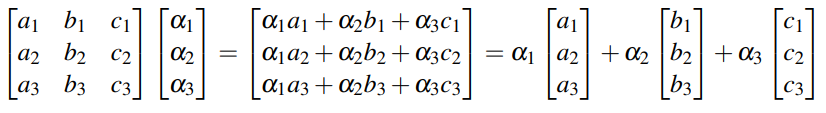
- The sum term says that, in other words, matrix-vector multiplication is a linear combination of columns:
Theorem 3.2 #
If the columns of .$A$ in the system of linear equations .$A\vec x = \vec b$ are linearly dependent, then the system does not have a unique solution.
- Start by assuming we have a matrix A with linearly dependent columns
$$A = \begin{bmatrix} | & | & & | \\ \vec a_1 & \vec a_2 & \dots & \vec a_n \\ | & | & & | \\ \end{bmatrix}$$
- By the definition of linear dependence, there exist scalars .$\alpha_1, \dots, \alpha_n$ such that .$\alpha_1\vec a_1 + \dots + \alpha_n \vec a_n = \vec 0$ where not all of the .$\alpha_i$’s are zero. We can put these αi’s in a vector:
$$\vec \alpha = \begin{bmatrix} \alpha_1 \\ \vdots \\ \alpha_n \\ \end{bmatrix}$$
- By the definition of matrix-vector multiplication, we can compactly write the expression above:
$$A\vec \alpha = \vec 0$$ $$\text{where } \vec \alpha \neq \vec 0$$
- Recall that we are trying to show that the system of equations .$A\vec x = \vec b$ does not have a unique solution. We know that systems of equations can have either zero, one, or infinite solutions.
- If our system of equations has zero solutions, then it cannot have a unique solution, so we don’t need to consider this case.
- Now let’s consider the case where we have at least one solution, .$\vec x$:
- Therefore, .$\vec x + \vec \alpha$ is also a solution to the system of equations! Since both .$\vec x$ and .$\vec x + \vec \alpha$ are solutions, and .$\vec \alpha \neq \vec 0$, the system has more than one solution. We’ve now proven the theorem.
$$A \vec x = \vec b$$ $$A \vec x + \vec 0= \vec b$$ $$A \vec x + A \vec \alpha = \vec b$$ $$A (\vec x + \alpha) = \vec b$$
Note that we can add any multiple of .$\alpha$ to .$\vec x$ and it will still be a solution – therefore, if there is at least one solution to the system and the columns of .$A$ are linearly dependent, then there are infinite solutions.
- Intuitively, in an experiment, each column in matrix .$A$ represents the influence of each variable .$x_i$ on the measurements. If the columns are linearly dependent, this means that some of the variables influence the measurement in the same way, and therefore cannot be disambiguated. See page five for good example.
Implications: #
This result has important implications to the design of engineering experiments. Often times, we can’t directly measure the values of the variables we’re interested in. However, we can measure the total weighted contribution of each variable. The hope is that we can fully recover each variable by taking several of such measurements. Now we can ask: “What is the minimum number of measurements we need to fully recover the solution?” and “How do we design our experiment so that we can fully recover our solution with the minimum number of measurements?”
Consider the tomography example. We are confident that we can figure out the configuration of the stack when the columns of the lighting pattern matrix .$A$ in .$A\vec x = \vec b$ are linearly independent. On the other hand, if the columns of the lighting pattern matrix are linearly dependent, we know that we don’t yet have enough information to figure out the configuration. Checking whether the columns are linearly independent gives us a way to validate whether we’ve effectively designed our experiment.
Row Perspective #
Optional!
- Intuitively, each row represents some measurement
- If the number of measurements taken is at least the number of variables and we cannot completely determine the variables, then at least one of our measurements must be redundant (it doesn’t give us any new information).
- This intuition suggests that the number of variables we can recover is equal to the number of unique measurements, or the number of linearly independent rows – this formal proof will come in a later note when we talk about rank.
- Now have two perspectives: in the matrix, each row represents a measurement, while each column corresponds to a variable.
- Therefore, if the columns are linearly dependent, then we have at least one redundant variable.
- From the perspective of rows, linear dependency tells us that we have one or more redundant measurements.
Span #
- Span of the columns of .$A$ is the set of all linear combinations of vectors .$\vec b$ such that .$A\vec x = \vec b$ has a solution
- .$\exists \vec x$ s.t. .$A \vec x = \vec b \Longrightarrow \vec b \in \text{span(cols}(A))$
- That is, the set of all vectors that can be reached by all possible linear combinations of the columns of .$A$
- Formally, .$\text{span}(\vec v_1, \dots, \vec v_N) = \bigg\{\sum_{i=1}^N \alpha_i \vec v_i\ |\ \alpha_i \in \mathbb{R},\ \vec a_i \in \mathbb{R}^{M}\bigg\}$
- A set of vectors is linearly dependent if any one of the vectors is in the span of the remaining vectors.
- That is, if any one of the vectors could be represent as the combination of the remaining vectors (that is, it’s in the span of the others)
- On the other hand, if each vector adds another dimension to the span (contains novel information) then they’re said to be linearly independent
- span, range, and column space of .$A$ all refer to the span of the columns of .$A$
Two Examples
- e.x. what is the span of the cols of .$A = \begin{bmatrix} 1 & 1 \\ 1 & -1\\ \end{bmatrix}$? $$\text{span(cols of A)} = \bigg\{ \vec v\ |\ \vec v = \alpha \begin{bmatrix} 1\\ 1\\ \end{bmatrix} + \beta \begin{bmatrix} 1\\ -1\\ \end{bmatrix}; \alpha, \beta \in \mathbb{R}\bigg\} = \mathbb{R}^{2}$$
- e.x. what is the span of the cols of .$A = \begin{bmatrix} 1 & -1 \\ 1 & -1\\ \end{bmatrix}$? $$\text{span(cols of A)} = \bigg\{ \vec v\ |\ \vec v = \alpha \begin{bmatrix} 1\\ 1\\ \end{bmatrix}; \alpha \in \mathbb{R}\bigg\} = \text{line } (x_1 = x_2)$$
02-03: Intro to Circuit Analysis #
Our ultimate goal is to design systems that solve people’s problems. To do so, it’s critical to understand how we go from real-world events all the way to useful information that the system might then act upon. The most common way an engineered system interfaces with the real world is by using sensors and/or actuators that are often composed of electronic circuits; these communicate via electrical signals to processing units, which are also composed entirely of electronic circuits. In order to fully understand and design a useful system, we will need to first understand Electrical Circuit Analysis.
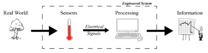
- There are four main steps involved when designing information devices and systems
- Analog World
- Sensor Input
- Data Processing
- Actuation (16B)
Tiny Bit of Solid-State Physics #
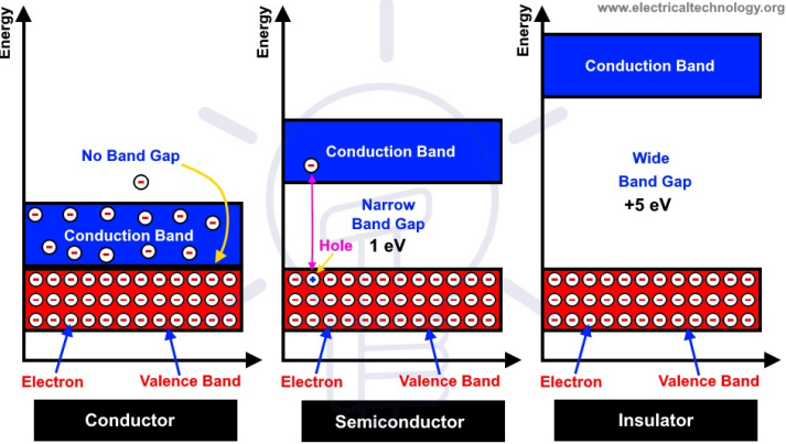
- Conductors have lots of electrons
- Move around very easily
- E.x. copper, gold, silver, water
- Conductors have lots of electrons
- But they are at an energy level where they need to be given some energy level (e.x 1 eV) to move
- E.x. solar cell, diodes
- Insulators do not let electrons pass through them
- E.x. capacitors have a big insulator in the middle, that is, current only goes through a capacitor when the magic smoke is released
Electrical Quantities #
| Quantity | Symbol | Units | What |
|---|---|---|---|
| Current | .$I$ | Amps, .$A$ | Flow of charges (e.g. electrons) in the circuit due to a potential difference |
| Voltage | .$V$ | Volts, .$V$ | Potential energy (per charge) between two points in the circuit |
| Resistance | .$R$ | Ohms, .$\Omega$ | Material’s tendency to resist the flow of current. |
- Voltage .$\pm$ depends on reference point
- Voltage, or electric potential, is only defined relative to another point (mountain/height analogy).
- Similarly, in circuits, we will frequently define a reference point, called ground, against which other voltages can be measured.
- Current .$\pm$ depends on direction
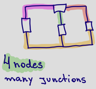
Circuit Diagram #
- Collection of elements, where each element has some voltage across it and some current through it
- Two main elements:
- Notes: Points where elements meet
- Junctions: Points where different material meet
- Voltage = difference of two potential
Basic Circuit Elements #
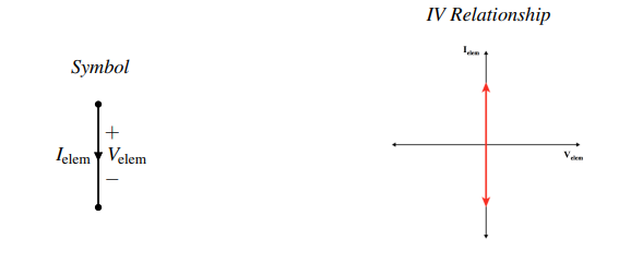
Wire #
- The most common element in a schematic is the wire, drawn as a solid line The .$IV$ relationship for a wire is:
- .$V_\text{elem} = 0$: A wire is an ideal connection with a constant, zero voltage across it.
- .$I_\text{elem} = ?$: The current through a wire can take any value, and is determined by the rest of the circuit.
Resistor #
- The .$IV$ relationship of a resistor is called Ohm’s Law:
- .$V_\text{elem} = I_\text{elem} R $: The voltage across a resistor is determined by Ohm’s Law.
- .$I_\text{elem} = V_\text{elem} / R$: The current through a resistor is determined by Ohm’s Law.
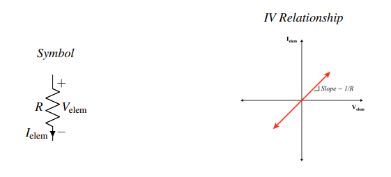
Limit check
- The slope is proportional to .$R^{-1}$, that is, the larger the resistance the lower the slope
- .$\lim_{R \to 0}$ results in an wire (above)
- .$\lim_{R \to \infty}$ results in an open circuit (below)
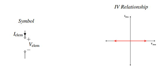
Open Circuit: #
- This element is the dual of the wire.
- .$V_\text{elem} = ?$: The voltage across an open circuit can take any value, and is determined by the rest of the circuit.
- .$I_\text{elem} = 0$: No current is allowed to flow through an open circuit; always zero.
Voltage Source: #
- A voltage source is a component that forces a specific voltage across its terminals. The + and − sign indicates which direction the voltage is pointing. The voltage difference between the “+” terminal and the “−” terminal is always equal to Vs, no matter what else is happening in the circuit.
- .$V_\text{elem} = V_S$ – The voltage across the voltage source is always equal to the source value.
- .$I_\text{elem} = ?$ – The current through a voltage source is determined by the rest of the circuit.

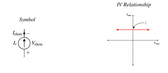
Current Source: #
- A current source forces current in the direction specified by the arrow indicated on the schematic symbol. The current flowing through a current source is always equal to Is, no matter what else is happening in the circuit. Note the duality between this element and the voltage source.
- .$V_\text{elem} = ?$ – The voltage across a current source is determined by the rest of the circuit.
- .$I_\text{elem} = I_S$ – The current through a current source is always equal to the source value.
Rules for Circuit Analysis #
- See also: 26.3 Kirchhoff’s Rules
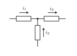
Kirchhoff’s Current Law (KCL) #
- Node: A place in a circuit where two or more of the above circuit elements meet
- The net current flowing into/out-of any node is zero: $$(-i_1)+(-i_2)+i_3 = 0$$
- That is, the current flowing into a node must equal the current flowing out of that node $$ i_1+i_2=i_3$$
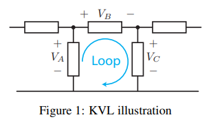
Kirchhoff’s Voltage Law (KVL) #
- The sum of voltages across the elements connected in a loop must be zero
- Mathematically, KVL states that: $$\sum_\text{loop} V_k = 0$$ $$\Longrightarrow V_A - V_B - V_C = 0$$
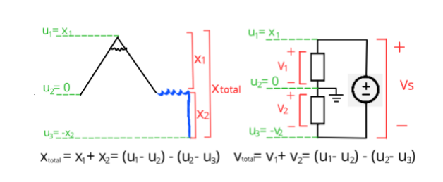
Height Analogy #
If you walk in a circle (a loop) so that you end up back where you started, than your total change in elevation must be zero, no matter how much you go up or down. If you walk in a line, ending up somewhere different, than your total change in elevation is equal to the sum of all of the elevation changes along the way.
Real World Analogy The sum of voltages across the elements connected in a loop must be equal to zero “what goes up must come down” If the arrow corresponding to the loop goes into the “+” of an element, we subtract the voltage across that element. We went “downhill” from higher voltage to lower voltage so we lost “elevation.” If the arrow goes into the “-” of an element, we add the voltage across that element This is like going “uphill”
Ohm’s Law and Resistors #
$$V_\text{element} = I_\text{element}R$$
- The unit of .$R$ is Volts/Amperes, called Ohms .$\Omega$.
- See also: 25.3 Ohm’s Law: Resistance and Resistors